A thesis presented for the degree of Doctor of Philosophy
in Economics
at
the University of Canterbury Christchurch, New Zealand
by
CONTENTS
CHAPTER PAGE
1.
ABSTRACT • • . • • • • • • • • . • . • . • • • . • •• 1
INTRODUCTION . •
1. Introductory comments
2. An outline of the thesis •
3. Conventions used in the thesis .
3
3
4 6
2. A CRITICAL EXAMINATION OF THE NORMALITY
ASSUMPTION IN THE LINEAR REGRESSION MODEL 8
8
9
1. Introduction
2. The Gaussian law of error
3. The relevance of the normality assumption
in an economic context •
4. Concluding remarks • . •
3. SPHERICALLY SYMMETRIC AND ELLIPTICALLY SYMMETRIC
DISTRIBUTIONS: A REVIEW OF THE LITERATURE •
· 12
· 18
21
1. Introduction. • •• • . • • • 21
2. Definitions and examples
3. Elliptically symmetric random vectors
. . • 21
• 26
4. Spherically invariant stochastic processes . . 34
5. Spherical matrix distributions . . • . • • 36
6. A summary of the important properties of
CHAPTER PAGE
4. STATISTICAL PROPERTIES OF LEAST SQUARES REGRESSION
ESTIMATORS WHEN DISTURBANCES ARE ELLIPTICALLY
SYMMETRIC • • • • • • • • • • • 42
1. Introduction • • • • • • • • • • • • • • • • • 42
2. Weak consistency of least squares
regression estimators • • • • • • • • 44
3. Strong consistency of least squares
regression estimators
4. Asymptotic distributions of least squares
regression estimators
5. An alternative to the Gauss-Markov theorem
for elliptically symmetric disturbances
Maximum likelihood estimation
• • • • 59
· . • • 73
75
• 82
6.
7. Conclusions . • • . . . • . . 88
5. SMALL SAMPLE PROPERTIES OF TESTS AND ESTIMATORS
WHEN THE REGRESSION DISTURBANCES ARE ELLIPTICALLY
SYMMETRIC
1. Introduction
2. A theoretical result
3. Implications for the validity of statistical
tests
90
• • 90
· 91
· 96
4. Power properties of tests for serial correlation
and heteroscedasticity • • • • .103
5. The distribution of statistics not invariant to
the scale of the disturbances
6. The dist.ribution of regression estimators
7. Conclusions
· . . .1l8
.128
CHAPTER PAGE
6. TESTING FOR AUTOCORRELATION USING LINEAR UNBIASED
REGRESSION RESIDUALS WITH SCALAR COVARIANCE MATRICES . 137
1. Introduction • • • 137
2. Testing for a given characteristic matrix of
regression disturbances 140
3. Testing for autocorrelation using LUS residuals • 150
4. Discussion. •
5. Conclusions
7. THE DURBIN-WATSON BOUNDS TEST AND REGRESSIONS
THROUGH THE ORIGIN •
1. Introduction • •
2. Pre-test bias considerations
• • 158
163
165
. . . • • 165
• 167
3. The powers of the alternative procedures . 168
4. Bounds for testiny ~or negative autocorrelation • 173
5. Conclusions
8. TESTING FOR MOVING AVERAGE DISTURBANCES IN THE
LINEAR REGRESSION MODEL
1. Introduction. •
• 178
179
. • • 179
2. An optimal power property of the DW test against
MA(l) disturbances • • 181
3. A new test for MALI) disturbances • • 187
4. A comparison of power properties of the two tests. 193
5. Conclusions 202
9. SUMMARY AND CONCLUSIONS • . • • • • • . • • . • • • • 203
PAGE
REFERENCES • • • . • • . • • • • . • . . • . . . . • • 210
APPENDIX 1: ARTIFICIALLY GENERATED TIME SERIES
DATA USED IN CHAPTERS 7 AND 8 • . • • • . 227
APPENDIX 2: AN EVALUATION OF THE NORMAL PSEUDO-RANDOM NUMBER GENERATOR USED IN THIS THESIS
1. Introduction 2. Results .
3. Choice of generator . .
229 229
236
LIST OF TABLES
TABLE PAGE
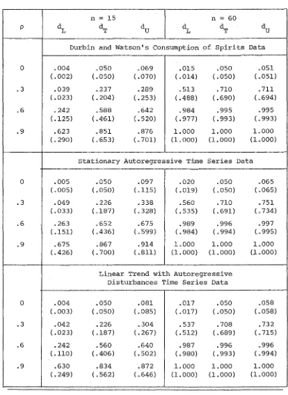
7.1 Powers of the Durbin-Watson bounds and the exact Durbin-Watson test using Kramer's procedure (and
Durbin and Watson's procedure) • 174
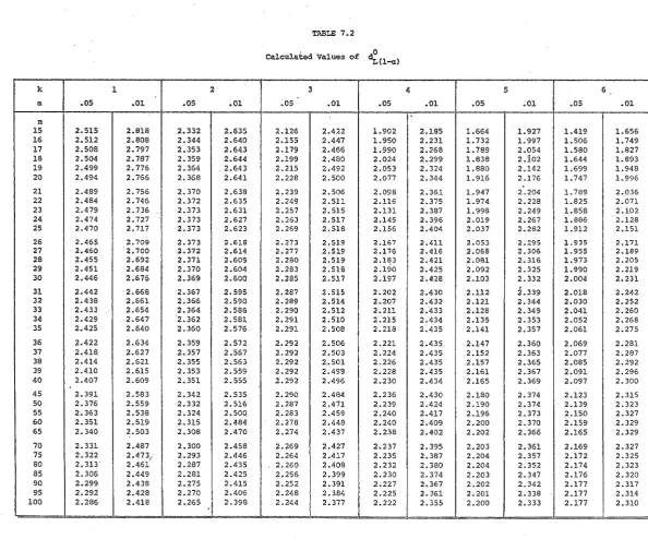
7.2 Calculated values of • 177
8.1 Five percent critical values of the one-tailed
F test • • • • 196
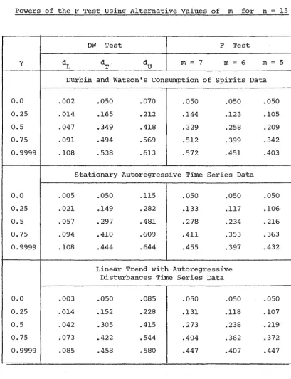
8.2 Powers of the DW test using alternative critical values and powers of the F test using alternative
values of m for n
=
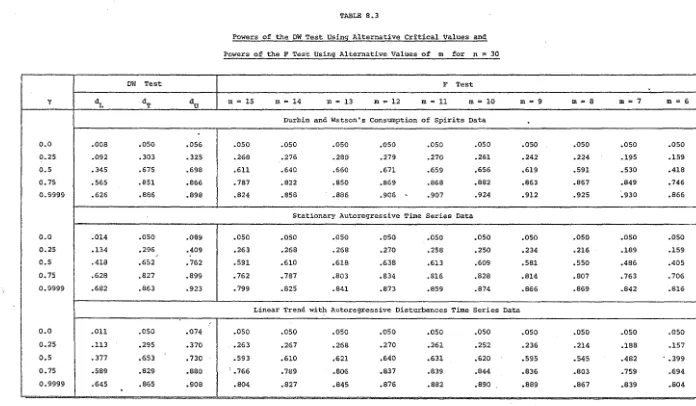
15 • • • 1978.3 Powers of the DW test using alternative critical values and powers of the F test using alternative
values of m for n
=
30. . .
.
.
.
. . ·
· ·
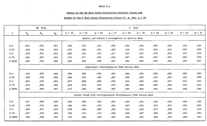
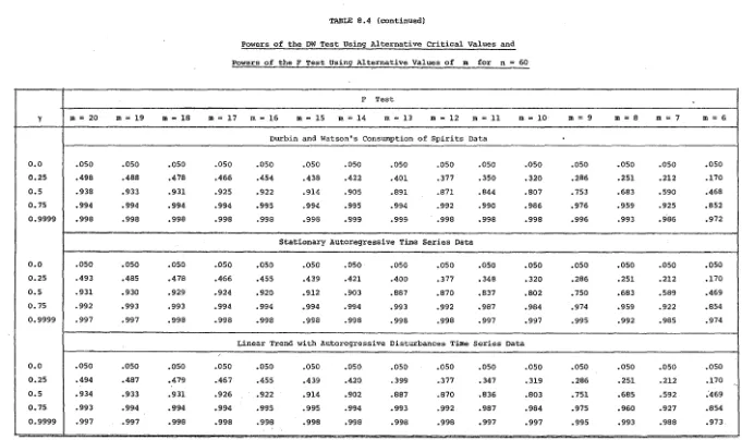
• 198 8.4 Powers of the DW test using alternative criticalvalues and powers of the F test using alternative
values of m for n
=
60 199LIST OF FIGURES
FIGURE PAGE
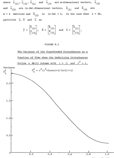
8.1 The variance of the transformed disturbances as a
function of time when the underlying disturbances
2
ABSTRACT
This thesis considers two aspects of statistical inference associated with the linear regression model set in an economic context. The implications of replacing the conventional normality assumption with the broader assumption that the disturbances follow an elliptically symmetric distribution, are investigated, and three features of the problem of detecting serial correlation in elliptically symmetric disturbances, are studied.
An examination of the conventional justification of the normality assumption in econometrics, conducted in Chapter 2, provides motivation for the study of regression analysis under the elliptical symmetry assumption.
Chapter 6 attempts to find an "optimal" test for first-order
autoregressive disturbances based on LUS residuals. A test, which
is optimal for certain design mat:t;:"ices, is constructed and shown to
be the Abrahamse-Koerts test.
Durbin and Watson's and Kramer's procedures for applying the
Durbin-Watson test to a regression equation without an intercept,
are compared in Chapter 7. While being susceptible to pre-test
bias, Kramer's procedure is found to have superior power.
Chapter 8 considers the problem of detecting first-order moving
average disturbances. The Durbin-Watson test is shown to be
approx-imately locally best'invariant. A new test is proposed and found to
CHAPTER 1
INTRODUCTION
1. INTRODUCTORY COMMENTS
The underlying philosophy of this thesis is provided by the
following two fundamental propositions:
(i) The usefulness of any theory of statistical inference depends
on, amongst other things, the generality of the assumptions
upon which the theory is based.
(ii) With respect to a problem of hypothesis testing, it is
desirable that full regard be given to the power properties
of the resultant test when the choice of test procedure is
made.
This thesis makes a number of contributions, in the spirit of (i) and
(ii), to the classical theory of statistical inference associated with
the linear regression model set in an economic context.
There is a growing body of evidence which suggests that, the
assumption of normally distributed disturbances, that underlies much
of the classical theory, may often be an unrealistic one. A review of
this evidence, together with a critical examination of the conventional
justification of normality, leads one to the conclusion that this
traditional assumption will frequently be violated in practice. This
provides motivation for wanting to consider a theory of inference based
on a wider class of disturbance distributions than that of multivariate
normal.
The major portion of the thesis is therefore devoted to determining
replacing the normality assumption with the wider, and perhaps more
acceptable assumption that the regression disturbances follow an
elliptically symmetric distribution.
Some of the results of this inquiry are used in the second part
of the thesis where three aspects of the problem of testing for serial
correlation in elliptically symmetric regression disturbances are
investigated in the spirit of proposition (ii). In this part of the
thesis, an attempt is made to find an "optimal" exact test for
first-order autoregressive disturbances, the question of applying the
Durbin-Watson bounds test to a regression fitted throught the origin is
discussed, and the potential of the Durbin-Watson test as a test
for first-order moving average disturbances is explored.
2. AN OUTLINE OF THE THESIS
Chapter 2 briefly reviews the controversy surrounding the "Gaussian
law of error" as a theory of measurement error, and then critically
examines the validity of the normality assumption in .the linear regression·
model, set in an economic context, from both a theoretical and an empirical
point of view.
Definitions of spherically symmetric and elliptically symmetric
distributions are given in Chapter 3. This is followed by a survey of
the literature concerned with the properties of these distributions.
The chapter closes with a summary of those properties which are used
elsewhere in the thesis.
The subsequent two chapters investigate various aspects of statistical
disturbances. In Chapter 4, a number of properties of the ordinary
least squares and the generalized least squares estimators of regression
coefficients are established. Conditions are given for weak consistency
and strong consistency of both estimators, and their asymptotic
distributions are discussed. The generalized least squares estimator
is shown to satisfy a stringent, and intuitively desirable, optimality
property, as well as being the maximum likelihood estimator. l
The size and small sample power properties of the numerous
statistical tests associated with the classical linear regression
model are investigated in Chapter 5. 2 The results established in
this chapter also enable the distributions of regression parameter
estimators to be related to their distributions for normally distributed
disturbances. The first half of the chapter considers the small sample
distributions of regression statistics which are invariant to the scale
of the disturbances, while the latter half deals with the distributions
of arbitrary statistics for a restricted class of elliptically symmetric
disturbances.
Chapter 6, 7 and 8 each consider different aspects of the problem
of testing for serial correlation in elliptically symmetric regression
disturbances.
1. For a slightly restricted class of elliptically symmetric disturbance distributions.
2. A paper presenting some of the author's preliminary results
concerning the optimality of various tests for serial correlation in elliptically symmetric regression disturbances, has been
Chapter 6 begins by briefly reviewing that part of the large
body of econometric literature on the subject of testing for serial
correlation which is concerned with the construction of exact tests
as alternatives to the Durbin-Watson bounds test. A number of
empirical investigations suggest that the small sample properties
of most of these tests are distinctly inferior to those of the
Durbin-Watson test. A possible explanation is that proper r~gard was not
given to the potential power of these exact tests in their construction.
Chapter 6 reports an attempt to find the "optimal" exact test based on
linear unbiased residuals with a scalar covariance matrix.
Chapter 7 considers the problem of applying the Durbin-Watson
bounds test to a regression equation fitted through the origin. The
small sample power properties of the procedure suggested by Durbin
and Watson (1951~ and an alternative procedure proposed by Kramer
(1971) are compared. The possibility of pre-test bias in the latter
is discussed and Kramer's procedure is extended in order to test for
negative autocorrelation.
The potential of the Durbin-Watson test, as a test for first-order
moving average disturbances, is investigated in Chapter 8. It is found
to be an approximately locally best invariant test. A new exact test
for first-order moving average disturbances is proposed and the small
sample power properties of the two tests are compared for selected
design matrices.
Concluding remarks are made in Chapter 9.
3. CONVENTIONS USED IN THE THESIS
Throughout this thesis, upper case characters are used to denote
and vectors. In keeping with current practice in econometrics, no
attempt is made, by the use of symbols, to distinguish between a
random variable or vector and the value taken by that random variable
or vector.
The term "orthogonal" has two meanings depending on its context.
An
orthogonal
matrix is defined as a non-singular matrix whose transposeis its inverse. On the other hand, a set of non-zero vectors, {xl, ••• ,xn}, is defined to be
orthogonal
ifx~x.
=
0,~ J for i,j=l, ••• ,n,ifj.
An orthogonal set of vectors is orthonormal, if and only if all vectors .
have unit length; i.e., if and only if
x~x ..
CHAPTER 2
A CRITICAL EXAMINATION OF THE NORMALITY ASSUMPTION IN THE LINEAR REGRESSION MODEL
1. INTRODUCTION
The assumption of normally distributed disturbances underlies much of the classical theory of statistical inference associated with the linear regression model. The aim of this chapter is to critically examine the relevance of this assumption for the linear regression model set in an economic context.
Over the past century, the role of the normal distribution in statistics has increasingly become a matter of controversy. This controversy is briefly reviewed in Section 2 and an attempt is made to clarify the issues involved. Historically, the emphasis has been on the role of the normality assmuption in problems in which the stochastic variability is solely due to measurement errors; the supposition that such errors are normally distributed being known as the Gaussian law of error. Section 2 closes with a discussion of the theoretical and empirical object.tons to the Gausstan law of error.
These objections do not necessarily apply to econometric models because the stochastic variability in such models typically has other causes besides measurement error. Section 3 critically examines the conventional justification for the normality assumption in econometrics. A number of theoretical objections are discussed and the empirical
2. THE GAUSSIAN LAW OF ERROR
Although the normal distribution is often named after Gauss, it
was first identified by De Moivrein 1733 as the limiting form of the
binomial distribution. Without reference to De Moivre's work, Gauss
(1809) rediscovered the normal distribution while formulating his
theory of measurement error. Gauss started from the premise that
when a number of equally good observations of an unknown quantity,
x, are given, the mean of the observations is generally accepted as
the most accurate estimate of x. Assuming independent observations,
he then found the only error distribution which satisfied his initial
premise was the normal distribution. In other words, Gauss constructed
the normal distribution to best suit the sample mean as an estimator
of x.
Despite this tenuous line of reasoning,l the case for the Gaussian
law of error was strengthened by Laplace (1812) who formulated the first
(incomplete) statement of the Central Limit theorem - that under general
conditions on the parent distribution, the distribution of the mean of
a random sample tends to normality as the sample size increases.
Unfort-unately, Laplace and a number of later writers tended to overstate the
generality of what had been proved. Statements were made in support of
the Gaussian law of error implicitly assuming that the parent distribution
of a random sample converges to a normal distribution as the sample size
increases. 2 An example of such an implicit assumption may be found in
1. Evidence which demonstrates that the sample mean was not universally accepted in Gauss's time may be found in survey articles by Huber
(1972) and Harter (1974a). Gauss, himself, admitted in 1823 that his earlier reasoning was not entirely satisfactory.
Laplace's (1812) claim3 that for Gauss's problem,the best method of estimating x depends on the particular form of the law of error when the number of observations is small, but is the arithmetic mean when the sample size is large.
About this time, Poisson (1824) discovered that for the Cauchy distribution, the mean of a random sample follows the same distribution law as the parent distribution. Hagen (1837) and Bessel (1838) made a significant contribution to the understanding of the conditions required for Gaussian errors by developing their "Hypothesis of Elementary
Errors". Their starting postulate was that the total error committed in any physical measurement is the sum of a large number of mutually independent elementary errors, each with the same absolute magnitude and equal probabilities of being positive or negative. The Central Limit theorem then implies that the total error is approximately normally distributed. Both Hagen and Bessel warned against the blind acceptance of the Gaussian law OI error.
Despite such warnings and Poisson's discovery, for the greater part of the nineteenth century the Gaussian law of error enjoyed almost universal acceptance. The attitude of this era is perhaps
best summed up in the following remark which Poincare (1912) attributes to Lippman:
"Everybody believes in the law of errors, the experimenters because they think it is a mathematical theorem, the mathematicians because they think it is an experimental fact."
Cramer (1946, p.231) writes of the years following the publication of the works of Gauss and Laplace:
"It was for a long time more or less regarded as an axiom that statistical distributions of practically all kinds would approach the normal distribution as an ideal limiting form, if only we could dispose of a sufficiently large number of sufficiently accurate observations. The deviation of any random variable from its mean was regarded as an 'error', subject to the 'law of errors' expressed by the normal distribution."
Against this background, a number of eminent scientists of the
day, such as Dirichlet, Hagen, Bessel, Laurent, Edgeworth, Poincare,
Newcomb and Charlier, began to question the universal and indiscriminate
use of the Gaussian law of error. 4 Also, a slow trickle of empirical
studies consistently showed that observed measurement errors appear to
follow distribution laws in which larger errors occur with a higher
probability than predicted by the normal distribution. For example,
Bessel (1818) observed three empirical error distributions exhibiting
such tendencies, but considered the discrepancies from the normal law
to be insignificant. Newcomb (1886) studied the empirical distribution
of 684 measurements of an angle dGj found the frequency of occurrence
of large errors to be greater than that predicted by the Gaussian law.
He boldly stated (p.346) that such empirical distributions "must be the
case in nearly all astronomical and physical work". For other empirical
examples of measurement errors following distributions with fatter tails
than the normal distribution, see Jeffreys (1948, Ch. 5.71, and references
;tn Hampel (1973, p.88) and Hsu (1979).
Newcomb (1886), Eddington (1933) and Jeffreys (1938) also raised
theoretical objections to the Gaussian law of error. They argued that
4. See Harter (1974a, 1974b) for a review of the controversy surrounding the Gaussian law of error. Also see S~rndal (1971) for a more
even if one accepts the hypothesis that the error of any given
measure-ment is normally distributed, the variance of such errors will most
likely differ from observation to observation. This could occur as
a consequence of the data being collected either by a number of
observers of differing skill or by the same observer working under
varying conditions. Lack of knowledge about how the error variance
changes from measurement to measurement allows one to view the variance
of individual errors as a random variable. The observed distribution
of such error therefore will have a probability density function of
the form
(2.2.1) f (x)
where F(T) is a distribution function supported on [o,oo}. If, for
example, F(T) is an inverted gamma distribution function, then
(2.2.1) is the density function of a Student's t distribution.
Members of this latter class of error distribution have been preferred
as alternatives to the Gaussian law of error by GeffLeys (1948) and
Anderson and Ellis (1971).
3. THE RELEVANCE OF THE NORMALITY ASSUMPTION IN AN ECONOMIC CONTEXT
The discussion so far has centred on problems in which the stochastic
variability is solely due to measurement error. This thesis is concerned
with the theory of statistical inference in the linear regression model
(2.3.1)
y
=
xS
+ u,where y is an n-dimensional random vector, X is an n x k matrix of observations on k nonstochastic variables,
S
is a k-dimensionalrandom disturbances. In the majority of economic applications,
measure-ment error will only be one of many possible causes of stochastic
variability in (2.3.1).
Haavelmo (1944) argued that random disturbance terms of econometric
models can be considered to be the sum of a large number of independent,
small, elementary random shocks and, therefore, will be approximately
normal. This line of reasoning has become the standard justification
for the normality assumption in econometrics. In this section we
critically examine its validity.
Johnston (1972, pp.lO-ll) gives the following three reasons for
including a disturbance term in the linear regression model, (2.3.1):
(i) It captures the effects on the endogenous variable of variables
not included in the model.
(ii) It allows the element of arbitrariness of human decisions to
be included in the model.
(iii) It takes account of any error in the measurement of the
endogenous variable.
The linear regression model (2.3.1) may be viewed as a simple
approx-imation to a more complicated and perhaps nonlinear model. This leads
to a fourth rationale for the inclusion of the disturbance term:
(iv) It allows one to take account of any discrepancy between the
true and the approximating models.5
Whether disturbance terms can always be expressed as sums of many
independent random shocks, is by no means clear. It seems reasonable
5. (i)-(iv) are not necessarily mutually exclusive.
to assume that they can be expressed as functions of independent random
shocks, but need such functions always be linear?
Assuming these functions are linear (or approximately linear), we
shall now consider whether, via the Central Limit theorem, this implies
the disturbances are approximately normally distributed.
The following is a statement of the Central Limit theorem due to
Lindeberg (1922):
Theorem 2.1: (Lindeberg Central Limit theorem) • Let
mutually independent random variables with distribution functions,
Fl , F2 , ..• , respectively, such that
E(z,) 0, 1.
Let
2 s n
Var(z, )
1.
and assume that for each E > 0,
(2.3.2) lim.l:...-
~
n-tro s2 i=ln
2 =
a.,
,1.
... + (J 2 n
Then the distribution of the normalized sum,
(2.3.3) s* n
=
(zl+"'+z )/s , n no.
tends to the standard normal distribution as n + 00
i=l, 2, •• , •
The so-called Lindeberg condition, (2.3.2), implies that for arbitrary E > 0 and n sufficiently large,
(2.3.4) for k=l, •.• , n.
is a measure of the variation contributes to the total variation of (2.3.3). Thus (2.3.4) may be described as stating that, asymptotically, (2.3.3) is the sum of many infinitesimal individual random shocks.
Note that (2.3.2) is not a necessary condition. The problem of whether necessary and sufficient conditions exist for the convergence of normalized sums, such as (2.3.3), to the standard normal distribution, to the author's knowledge, remains unsolved. Feller (1971) has shown
(2.3.2) to be necessary in the following sense:
Theorem 2.2. (Feller) If s ~ 00 and cr /s ~ 0 as n ~ 00 then the
n n n
Lindeberg condition, (2.3.2), is necessary for the convergence of (2.3.3) in distribution to a standard normal random variable.
Returning to our original problem of whether the disturbances of (2.3.1) can be regarded as being approximately normal, the first question we should ask is whether the independent random shocks, which sum to a disturbance term, satisfy the Lindeberg condition. Perhaps the most honest answer is that we cannot always be sure. One point is clear; it is likely that the degree of heterogeneity amongst the individual random shocks will be high. 6 Whether, in general, it is great enough to violate the Lindeberg condition is uncertain. Koenker and Bassett
(1978) argue that:
" it is rather puzzling that investigators, who are generally loathe to adopt informative priors about the systematic structure of their models about which theoretical considerations and past empirical experience should provide substantive evidence, should feel themselves so well informed about the unobservable con-stituents of their model's unobservable errors to argue that they satisfy a Lindeberg condition! A few gross errors occurring with low probability can cause serious deviations from normality: to dismiss the possibility of these occurrences almos.t invariably requires a leap of Gaussian faith into the realm of pure speculation."
Suppose we take such a "leap of Gaussian faith" and assume that th e L1n e erg con 1t10n 1S sat1s 1e • Intuitively, one could argue 'd b d' , 7, , f' d that the speed of convergence to the standard normal law will depend on the degree of homogeneity of the independent random shocks being summed; the more homogeneous the random shocks, the faster the convergence. For grossly heterogeneous random shocks, which may often be the case in econometrics, the approximation to normality may be extremely poor because of the slowness of convergence.
Even if for individual disturbance terms, the degree of approx-imation to normality is good, nothing in Haavelmo's theory guarantees the homogeneity of regression disturbances. If the disturbances of
(2.3.1) are normally distributed with differing variances and we are completely ignorant about how the variance changes from observation to observation, then we may view the variance of the disturbances as a random variable. In this case, the observed distribution of the disturbances will have a probability density function of the form
8
of (2.2.1).
7. Or some other sufficient condition for convergence to normality.
Finally, let us consider the assumption of independent disturbances
that often accompanies the normality assumption in classical regression
analysis. There is no special reason why disturbances should be
independent. When one considers both the dynamic and interrelated
nature of a modern economy, this assumption begins to look like
wishful thinking. As Lindley (1979) recently remarked, "it is hard
to find things that are tru!ly independent".
This point is well recognised by econometricians as the large
volume of literature concerned with the problem of serial correlation
in regression disturbances, attests. However, only for the normal
distribution does zero correlation between random variables necessarily
imply independence. The lack of evidence of correlation between
disturbances, therefore, should not always be interpreted as an
indication of independence. The convention of assuming independent
regression disturbances is perhaps a poor model for the physical world.
What does the available empirical evidence tell us about the
relevance of the normality assumption? There is a considerable
literature on the observed probability distributions of rates of
return on common stock in various countries. Mandelbrot (1963, 1967),
Fama (1963, 1965), Press (1967), Praetz (1972), Blattberg and Gonedes
(1974) and Praetz and Wilson (1978) all agree on one point - that such
distributions have fatter tails than predicted by the normal distribution.
Carlson (1975) found some empirical distributions of price expectations
displayed a similar tendency when he used survey data to test whether
price expectations are normally distributed. Granger and Orr (1972)
"Lately, there has been a growing awareness that some economic data display distributional characteristics that are flatly inconsistent with the hypothesis of normality. Frequency functions have been observed with too much mass near the mean and in the extreme tails, and not enough mass in the intervals between one and two standard deviations (roughly) from the mean •••. This pattern of behaviour holds true of time series and cross-section data alike, and has been observed for such widely disparate variables as stock and commodity price changes; sales, employment or asset size measures of business firms; and personal incomes."
On the other hand, Ramsey and Zarembka (1971) tested the normality assumption in five alternative specifications of a
u.s.
aggregateproduction function and found they could not reject any model solely on the basis of non-normality of the disturbances. In a similar study, Huang (1973) rejected the normality assumption of one model out of five. However, the tests used in both studies were not chosen because of their sensitivity to fat-tailed alternative distributions. This, together with the fact that approximately only 50 degrees of freedom were available for testing, suggests that these findings should not be regarded as a vindication of the normality assumption.
4. CONCLUDING REMARKS
The main response to this growing disenchantment with the normality assumption has been the development of a number of robust alternatives to the least squares estimator. This literature is reviewed by Huber (1972, 1973), Hampel (1973) and Harter (1974-1975). The widespread use of such estimation techniques has perhaps been hampered slightly by a lack of suitable statistical procedures for
9 conducting associated tests of hypotheses.
In the subsequent three chapters of this thesis, a different approach to the problem of non-normal disturbances is considered. We investigate the implications for the classical theory of regression analysis of replacing the normality assumption with the broader assumption that the regression disturbances follow an elliptically symmetric distribution.
This class of distributions was chosen for two reasons. First, a large subclass of elliptically symmetric distributions have univariate marginal distributions with probability density functions of the form of (2.2.1). This class of disturbance distributions, therefore, answers one of the theoretical objections to the normality assumption raised in
the previous section. Secondly, recent work by Zellner (1976),1° Kariya and Eaton (1977) and Kariya (1977) indicates that elliptically symmetric distributions possess properties which make them analytically tractable. These studies found that the Type I errors of the standard F tests and
9. Such statistical procedures are beginning to be developed. For example, see Bickel (1978).
Student's t tests of regression parameter values and the Durbin-Watson test, are invariant to a widening of the normality assumption to include appropriate elliptically symmetric disturbance distributions. Kariya showed that for a particular subclass of elliptically symmetric disturbance distributions, the Durbin-Watson test is an approximately uniformly most powerful invariant test for first-order autoregressive disturbances whenever the column space of the design matrix is spanned by k of the characteristic vectors of the first difference matrix, where k is the number of regressors. Clearly these results encourage further research.
CHAPTER 3
SPHERICALLY SYMMETRIC AND ELLIPTICALLY SYMMETRIC DISTRIBUTIONS: A REVIEW OF THE LITERATURE
1. INTRODUCTION
The purpose of this chapter is to introduce the reader to spherically symmetric and elliptically symmetric distributions. Definitions and examples are given in the next section and this is followed in subsequent sections by a review of the literature dealing with their various properties. We shall make use of many of these properties in later chapters. For this reason, the final section contains a convenient summary of the more useful properties that have been derived in the literature.
2. DEFINITIONS AND EXAMPLES
An n-dimensional random vector, x, has a spherically symmetric distributionl if its distribution laws are invariant to rotations about the origin, i.e. to orthogonal transformations. Clearly the distribution laws of such random vectors will be independent of direction from the origin and therefore will be a function only
k
of distance from the origin, namely i::
=
(x'x) 2 In particular this means that if x has a joint probability density function, it will be of the form(3.2.1) f (x) = ~ (x I x)
with respect to the Lebesgue measure on Rn, where
(3.2.2) and
(3.2.3)
~: [0,(0) -+ [0,(0)
-n/2
~r(n/2)'1f
Two alternative definitions of an n-dimensional spherically symmetric random vector used in the literature are: (i) a random vector which has a joint density function of the form of (3.2.1) and (ii) a random vector with a joint characteristic function of the form
(3.2.4) \jJ(t) = '!'(t't)
where '!' is some function on [0,(0) and t is an n-dimensional vector. The latter is equivalent to the definition given above while the former is more restrictive as it defines only those spherically symmetric distributions for which joint density functions exist.
Spherically symmetric distributions are members of a wider class of distributions which we shall call elliptically symmetric. 2 An n-dimensional random vector z has an elliptically symmetric distribution if its distribution laws are invariant to orthogonal transformations in the n-dimensional Euclidean geometry with the inner product
(u, v)
2. These distributions have also been called elliptical [Chu (1973)], spherically invariant [Vershik (1964)], elliptically contoured [DasGupta et ale (1972)] distributions and even occasionally spherically symmetric distributions [Goldman
where u and v are n-dimensional vectors and L is a given,
n x n, positive definite matrix. L is termed the characteristic
t . 3
ma rl.x.
Throughout this thesis the notation E(n,L) will be used to denote an n-dimensional elliptically symmetric distribution with characteristic matrix L. Obviously a spherically symmetric distribution is a special case of an E(n,L) distribution where
L = 02r and 02 is any positive scalar. Thus E(n,r) denotes n n an n-dimensional spherically symmetric distribution. Further, the notation
Z 'V E o (n,L)
will be used to denote that z is an E(n,L) random vector such that
Pr (z=O) O.
Clearly, if z is an E(n,L) random vector and S is any n x n, nonsingular matrix such that
S'S = L -1 I
then
(3.2.5) x = Sz
3. For any given elliptically symmetric distribution the characteristic matrix is uniquely determined up to a scalar factor. Wise and
has a spherically symmetric distribution. On the other hand, if x is an E(n,I) random vector with a joint density function of n the form of (3.2.1) and if A is an n x n non-singluar matrix then
(3.2.6) z = Ax
has a joint density function of the form
g (z)
I
A -11 ¢ (z' (A )' A z) -1-1(3.2. 7)
with respect to the Lebesgue measure on Rn where ~ = AA'. In
view of (3.2.5) and (3.2.6), if z is an E(n,~) random vector
with a joint density function, then this function will be of the form of (3.2.7) where
¢
is such that (3.2.2) and (3.2.3) hold.As in the spherically symmetric case, two alternative definitions of an E(n,~) random vector have been used in the literature. They
are: (i) a random vector which has a joint density function of the form of (3.2.7) and (ii) a random vector with a joint characteristic function of the form
(3.2.8) 1/1 (t) = II' (t' H)
where II' is some function on [0,00) and t is an n-dimensional
vector. Again the latter definition is equivalent to our definition while the former is more restrictive, defining only those elliptically
symmetric distributions for which joint density functions exist. 4
4. For a proof of the equivalence of (i) and (ii) in the case when a joint density function of the E(n,~) random vector is assumed
Any n-dimensional random vector with a joint density function of the form of (3.2.7) for some n xn positive definite matrix E is clearly elliptically symmetric. The class of elliptically symmetric
2
distributions includes the multivariate normal distribution, N(o,a E),
and the mUltivariate Student's t distribution with a joint density function of the form
(3.2.9) g(z)
where
p (v o )
a,v o >0, -oo<z.<oo, 1. i=l, ... ,n,
For v o > 2, and E = I , the elements of z are uncorrelated but n
not independent. When v o
=
1, (3.2.9) is a multivariate Cauchy density function for which no moments exist.An important class of elliptically symmetric distributions are those whose joint density functions can be expressed as mixtures of mUltivariate normal densities, i.e. as the Lebesgue-Stieltjes
integral,
(3.2.10) g (z)
=
J o 00 (2TIT ) 2 -n/2/ E exp{-z'E Z/2T }dF(T) /-~. -1 2where F(T) is any distribution function supported on [0,00). In fact for every elliptically symmetric density function of the form
(3.2.7) ,
is also an E(n,~) joint density function. Further examples of
elliptically symmetric distribu"tions have been given by Lord
(1954), McGraw and Wagner (1968), Chu (1973) and Goldman (1976).
The literature on elliptically symmetric distributions can
be classified into three groups: (i) papers investigating the
properties of E(n,~) random vectors, (ii) those that deal with
the class of spherically invariant stochastic processes; that is
stochastic processes whose n-dimensional marginal distributions
are E(n,~) and (iii) papers concerned with stochastic matrices
whose rows (or columns} are E(n,I n )i such matrices being labelled
spherical random matrices. Contributions in each of these three
branches of the literature are surveyed chronologically in the
following three sections.
3. ELLIPTICALLY SYMMETRIC RANDOM VECTORS
Early work on spherically symmetric distributions was done by
Maxwell (1860) who showed that independence of the components of
an E(n,I) random vector implied normality.5 n
Lord (1954) derived the joint characteristic function, ~(t),
of an E(n,I) random vector, x, with joint density function n (3.2.1); i.e.,
~(t)
=
JRn exp{ix't}~(x'x)dxwhere t is an n-dimensional vector. He found it to be the Hankel
transform:
(3.3.1)
. 1
where II til
=
(t't)"'2 and J m is the Bessel function of the first kind of mth order. Clearly 1jJ(t) is a function only of IItI!, henceconfirming that (3.2.4) holds when x has a joint density function.
Lord used this form of the characteristic function to show
that projections of spherically symmetric distributions onto spaces
of fewer dimensions are spherically symmetric and that when the
characteristic functions of distributions so related are expressed
in the form of (3.2.4), ~ takes a common form. He also demonstrated
that the sum of independent, not necessarily identically distributed,
E(n,I) random vectors is E(n,I). n n
The joint charaqteristic function of an E(n,I) random vector,
z, with. joint density of the form (3.2.7) is
(3.3.2)
Note that by applying the transformation (3.2.5) and following Lord's
proof for the spherically symmetric case, (3.3.2) can be shown to be
the Hankel transform (3.3.1) with II til = (t' It) ~ 2. This allows us to confirm that the joint characteristic function of an E(n,E) random
vector with joint density function (3.2.7) is of the form (3.2.8).
Box and Hunter (1957) found expressions for the moments of a
the one dimensional random walk generated by distance from the origin in Rn space when independent
are sununed.
E(n,I ) n random vectors
A number of significant contributions to the theory of elliptically symmetric distributions were made by Kelker (1970). He noted that a sufficient condition for the existence of the kth order moment of an E(n,E) random vector with joint density of the form (3.2.7) is that
(3.3.3) 00 k+n-l 2
fo r ~(r )dr < 00
6
holds. If (3.3.3) is satisfied for k = 1 then the mean of the E(n,E) random vector, z, is 0 while if it holds for k = 2, the covariance mat.rix of z is (J 2 is a positive scalar,
independent of E. In the case E
=
I , (J 2n is the variance of
each of the univariate marginal distributions.
Suppose z is an . E(n,E) random vector and that z and E are partitioned as
z
~
[:]where u and v have n-q and q components respectively and Ell and L22 are (n-q) x (n-q) and q x q respectively. Kelker
found the marginal density of v to be of the form
6. Note that if (3.3.3) holds for k
= kl it also holds for
(3.3.4) f(V)
for some function where is determined only by the form of and by q.Thus all marginal density functions of dimension q, q < n, have the same functional form. Further, he found that when E(ulv) exists,
(3.3.5) E(ulv)
In particular, this implies that if vector,
(3.3.6) E(ul v)
[~J
° .
is an E(n,I) n random
He also demonstrated that assuming the existence of a joint density function is not particularly restrictive. This was done by showing that all marginal distributions of an E (n,2:) o distribution have probability density functions. Therefore a sufficient condition
for an E(n,2:) distribution to have a joint density function is that it be a marginal distribution of an E o (n+1
,f)
distribution whereis any (n+l) x (n+l) positive definite matrix. Kelker generalized Maxwell's early result by showing that if E is a diagonal matrix, then independence of the components of an E(n,E) random vector, z, implies z has a N(O,a 2 2:) distribution. In addition he proved 7 that when {xn}:=l is a countable family of random variables, the joint distribution of any k of these variables is E(k,Ik) for each k, k=2, 3, ••• if and only if there is a non-negative random variable, T, such that conditional on the value taken by T, the
X 's are independent normal variables with mean zero and variance n ., i.e., the joint density has the form (3.2.10) with n = k and E
=
I k . A further property he reported is that if x is anE(n,I) random vector with a joint density function, then the n random variable
has a beta distribution with parameters (n-q)/2, q/2 .
Chu (1973) showed that if z is an E(n,E) random vector with
joint density function (3.2.7), there exists a scalar function w(s)
defined on (0,00) such that
fOO
o w(s)ds 1and (3.2.7) can be written as
(3.3.7) g (z)
where cp N (Z,L:jS) . =
s
n/2 (21f) -n/21 E I-~ exp{-sz'E z/2} -1 is the N(o,E/s) joint density function. Note that w(s) is not necessarily aprobability density function since it may take negative values. In
proving this result, Chu required
L-l[~(r)]
. 0 t eXls, were . t 8 hL-
lis the inverse Laplace transform operator. Hence (3.3.7) should not
be treated as necessarily holding for all E(n,E) random vectors
with joint density functions.
8.
~(r)
differentiable for sufficiently large r andrk~(r) ~
0Chu used (3.3.7) to demonstrate a number of properties of E(n,i:)
random vectors. For example, if m(z) is any Borel measurable function
of z for which E [m(z) ] exists .then
00
E[m(z)] =J w(s)E [m(z)]ds
o Ns
where EN [m(z)] is the expectation of m(z) assuming z to be s
N (0, i:/s) • Also if
( 3 • 3 • 8) u = Az
where A is an m x n matrix of rank m ~ n then the joint density
function of u is
00
h(u)
=
J o w(sH> (u,Ai:A'/s)ds N(3.3.9) =
I
Ai:A II
-~ 2cp (u U (ALA I) -1 u)m .
Note that h(u) has the same weighting function as g(z) in (3.3.7).
Thus the change in form of cp is caused by the change in the functional form of the normal density as the dimension changes from n to m.
(3.3.9) holds for transformations of any E(n,i:) random vector with
a joint density function and can also be obtained using (3.3.4).
Further, it is clear from the definition of elliptically symmetric
distributions that if z is an E(n,i:) random vector, not necessarily
with a joint density function, then u defined by (3.3.8) will be an
E (m,Ai:A I) random vector.
Goldman (1976) noted that the sum of two independent elliptically
symmetric random vectors with different characteristic matrices is not
two random vectors are normally distributed or when the two
characteristic matrices differ only by a scalar factor. He also
showed that if x is an E(n,I) random vector with joint density n function (3.2.1), there exists a unique set of random variables:
for which
(3.3.10)
Furthermore, r, 81 , density functions
(3.3.11)
rE [0,00),
8k E [0,1T] ,
8n_l E [0,21T)
xl rcos8 l , j-l
x. J r( IT sin8k)cos8. k=l J n-l
x n r IT sin8k k=l
k=l, ••• , n-2,
2::;j::;n-l,
.•. , 8 1 n- are independent and have respective
9 r E [0,00),
-~ -1 n-l-k
= r[(n-k+l)/2]1T [r[(n-k)/2]] sin 8k ,
1 /(21T) ,
8k E [O,1T] , k=l, • • 0 ,
8 1 E n- [0,21T) •
n-2,
Consequently, if r, 81, ••• , 8n_l are independent random variables " with density functions given by (3.3.11) then the random vector
defined by (3.3.10) is E(n,I ). n
A further consequence is that if x is an E(n,I) n random vector then its density function (if it exists) can be written as
f (x) = ~ (x I x)
where is the marginal density of distance from the origin.
This can be extended to the case where z is an E(n,I:) random
vector by making use of the transformation (3.2.5) so that
g(z)
1I:1-~~(z'I:-lz)
(2Tfn/2) -lr (n/2) II:
I-~PII
Szll [(z 'I:-lz)~]/
(z 'I:-lz) (n-l) /2where S is any n x n, nonsingular matrix such that SIS
Kariya and Eaton (1977) considered the distributions of
~ ~
-1 I: •
. ~
x/(x' x) ,
a'x/(x'x) 2 and x'Ax/(x'x) 2 where x is an E (n,I )
o n random vector,
a is an n-dimensional vector such that ala
=
1 and A is an n x n~
symmetric matrix. x/(xlx) 2 was shown to be uniformly distributed on
the n-dimensional, unit, hypersphere,
C n {xl x E R , n XiX
u.
~ 2 k
(n-l) 2w/(1-w ) 2, where w a'x/(x'x) ~ 2, was found to have a Student's ~
t distribution with n - 1 degrees of freedom. X'AX/(X'x) 2 was
shown to have the same distribution as
are the latent roots of A and
function,
n
jEldj y j where d " j =1, •.. , n, J have the joint density
n-l 2
with y = 1 - ,I:ly, n 1.= 1. In the special case when A = A and rank(A)
=
k, 1others who have made contributions to the theory of elliptically
symmetric distributions include Baldessari (1965), Ahmad (1972),
Das Gupta et ala (1972), Goldman (1972),Strawderman (1974), Wolfe
(1975), Ghosh and Pollak (1975), Crawford (1977) and Kariya (1977).
4. SPHERICALLY INVARIANT STOCHASTIC PROCESSES
A stochastic process may be regarded as an indexed set of random
variables, {xt ' t E T}, defined on a common probability space (Q,F,p)
A spherically invariant stochastic process is a stochastic process for
which the joint distribution of each finite arbitrary collection of the
Xt ' t E T, is elliptically symmetric. This class of stochastic process was first considered by Vershik (1964) who restricted his attention to
zero-mean, square integrable stochastic processes. He defined a process
to be spherically invariant if in the linear manifold generated by
arbitrary samples from the process, all random variables having the
same variance have the same distribution function. Blake and Thomas
(1968) established that this definition is equivalent to the former
definition in the restricted class of processes studied by Vershik.
Using the concept of semi-independency, Vershik found that his
class of spherically invariant stochastic processes is uniquely
characterized by the fact that every mean-square estimation problem
on the linear manifold generated by such a process has a linear
1 . 10
so utl.on. Two random variables, xl and x2' are semi-independent
10. The best mean-square estimator of Xt' t E T, given Xtl' •.• ,
0 0 1
Xtn; t l , .•• , tn E T, is the conditional expectation E[Xt Xt' ••. , Xt]. Every mean-square estimation problem has a linear~olu!ion
-n
I
if
E[x.lx.) 1. J E [x. ) 1. i,j=1,2,i~j,
or equivalently if each random variable is uncorrelated with any 11
arbitrary function of the other. Clearly from (3.3.6) the
components of an E(n,I ) n random vector whose second order moments exist are semi-independent. Vershik also demonstrated that his
class of spherically invariant processes is precisely that class
of processes for which the concepts of wide and narrow stationarity
are equivalent.
Yao (1973), who unlike Vershik did not restrict attention to
square integrable processes, proved that a process is spherically
invariant if and only if it is equivalent to a stochastic process
of the form {aYt' t E T} where a is a non-negative random variable and {Yt' t E T} is a zero-mean Gaussian stochastic process independent of a. Therefore any n-dimensional sample
from a spherically invariant stochastic process has a joint density
function12 of the form (3.2.10) where F(o) is the distribution
function of a. On the other hand, for a distribution to belong
to a finite dimensional sample from a stochastic process it must
t · f th K 1 . t d" 13 h
sa 1.S y e o mogorov cons1.S ency con 1.t1.ons so t at any E(n,L)
11. The concept of semi-independence lies between that of independence and being uncorrelated, in the sense that when second-order moments are assumed to exist, independence implies semi-independence and semi-independence implies zero correlation.
12. In view of Kelker's (1970) findings, joint density functions will exist for all such n-dimensional samples provided Pr(xt=O)
=
0 for all t E T.distribution is not necessarily the distribution of an n-dimensional sample from a spherically invariant process and hence need not have a joint density function of the form (3.2.10). Yao also noted that if {x, n ~ I} is a sequence of jointly spherically symmetric
n
random variables with finite second order moments, then
where is a martingale.
{z , n ~ I},
n
Yao's characterisation of spherically invariant stochastic processes was recently extended by Wise and Gallagher (1978) to
. 1 d . 1 14 . 1" . d
1nc u e s1ngu ar spher1cal y 1nvar1ant stochast1c processes an to allow a to be any real valued random variable independent of {Yt' t E T}. contributions to the theory of spherically invariant stochastic processes have also been made by Picinbono (1970) and Gualtierotti (1974, 1976).
5. SPHERICAL MATRIX DISTRIBUTIONS
Spherical matrix distributions have been studied by Maxwell (1860), Dempster (1969) and Dawid (1977). They are of interest because they arise naturally in certain applications, a prominant example being quantum theory [see Mehta (1967)]. Dawid defines an n x p random matrix, Y, to be left-spherical if its joint distribution is invariant to transformations of the form,
Y -+ UY
and right-spherical if its joint distribution is invariant to
transformations of the form
Y ~ YV
where U and V are nonstochastic orthogonal matrices of dimensions
(n x n) and (p x p) respectively. ClearlY, the columns of a
left-spherical random matrix and the rows of a right-left-spherical random
matrix are spherically symmetric.
Dawid investigated problems of inference about the parameters
of a multivariate linear model in which the usual assumption of
normality for the disturbances is replaced by the weaker assumption
that they follow an appropriate spherical matrix distribution. He
found that inference about parameter values and associated confidence
regions are identical to whatever is appropriate under normality.
6. A SUMMARY OF THE IMPORTANT PROPERTIES OF
ELLIPTICALLY SYMMETRIC DISTRIBUTIONS
Throughout this section, z denotes an E(n,L) random vector.
(I) If the joint density function of z exists, then it is of
the form
(3.6.1)
with respect to the Lebesgue measure on Rn where
~: [0,00) ~ [0,00)
(II) z is an E(n,~) random vector if and only if it has a
characteristic function of the form
where t is an n-dimensional vecto~ and ~ is a function
on [0,00) independent of ~.
(III) If A is an m x n matrix of rank m where m ~ n, then
Az is E(m,A~A'). In particular, all marginal distributions
of any elliptically symmetric distribution are elliptically symmetric. If z has a joint density function of the form of (3.6.1), then w
=
Az has a joint density function of the formf (w)
I
A~A
II-~~
(w I(A~A')
-lw)m
where ~m is determined only by the form of ~ and by m
and is such that
and
(:tv) If ~ is a diagonal matrix, independence of the components of z implies z has a multivariate normal distribution.
z
=
[:]
where u is (n-q) and v is q-dimensional, 0 < q < n, then
E[ulv] 0
(VI) If the first order moments of z exist
E[z]
=
0while if the second order moments exist, z has convariance
matrix
where cr 2
E[zz']
cr2~
is a positive scalar.
(VIr) The sum of indpendent, not necessarily identically distributed
elliptically symmetric vectors with characteristic matrices
which differ only by scalar factors, is elliptically symmetric.
(VIII) A sufficient condition for z to have a joint density function
is that it be a marginal distribution of an (n+l)-dimensional
elliptically symmetric distribution which does not have an atom
of weight at the origin.
(XI) A stochastic process is spherically invariant if and only if
it is equivalent to a stochastic process of the form {aYe t E T}
where a is a non-negative random variable, and {Yt' t E T} is a
zero-mean Gaussian stochastic process independent of a. The
characteristic function of an n-dimensional sample from a
(X)
tjJ n n (s ) = f 00 o exp(-v 2 s'L: s /2)dF(V) n n n
where s n is an n-dimensional vector, L: n is an n x n positive definite matrix and F(·) is the probability
distribution function of a. The sample's probability density function (if it exists) is of the form
h (z)
For any given spherically invariant process, F(·) is common
to all finite samples.
If x is an E (n,I) random vector then o n k
x/(x' x) 2
is uniformly distributed on the n-dimensional unit
hyper-sphere:
(XI) If x is an E(n,I) n random vector with a joint density fUnction of the form
f (x) <jJ (x' x) ,
there exists a unique set of random variables,
r E [0,00) , Ok E (o,'lf) ,
0n-1 E (0,2'lf),
for which
Xl
=
rcos81 ,x. J j=2, •.• ,n-l,
Furthermore, r, 81 , ... , 0n_l are independent and have respective density functions:
r E [O,do)
-~ -1 n-l-k
f[(n-k+l)/2]n 2[f[(n-k)/2]] sin 8k , Ok E [O,n] k=l, ... ,n-2
CHAPTER 4
STATISTICAL PROPERTIES OF LEAST SQUARES REGRESSION ESTIMATORS WHEN DISTURBANCES ARE ELLIPTICALLY SYMMETRIC
1. INTRODUCTION
The purpose of this chapter is to investigate some of the more important statistical properties of least squares estimators of 8
in the usual linear regression model,
y x8
+ U ,when the disturbance vector, u, is assumed to take an elliptically symmetric distribution.
Section 2 opens with a review of the literature on weak consistency of the OLS (Ordinary Least Squares) estimator of
8.
Then necessary and sufficient conditions are found for the weak consistency of linear "unbiased" estimators of8
assumingelliptically symmetric disturbances. We define such an estimator to be "unbiased 1,1 if it is, unbiased in the classical sense when
the dtsturbances have finite first order moments. The remainder of Section 2 is devoted to demonstrating the versatility of this result by applying it to the OLS, GLS (Generalized Least Squares) ~
instrumental variable and restricted least squares estimators of
8.
confined to the case of elliptically symmetric disturbances, sufficient
conditions are found for the strong consistency of the OLS estimator
under the classical assumption of uncorrelated disturbances. This
result allows us to obtain sufficient conditions for the strong
consistency of the GLS estimator when the disturbance covariance
matrix is known up to a scalar value; this being an important problem
which seems to have been ignored in the literature. Finally, necessary
and sufficient conditions are determined for the OLS estimator to be
strongly consistent assuming the regression disturbances are
elliptically symmetric with a diagonal covariance matrix and finite
second order moments.
The asymptotic distributions of the OLS and GLS estimators are
discussed briefly in Section 4. A powerful optimality property of
the GLS estimator when the regression disturbances are E(n,~) is
proven in Section 5. Without any assumption being made about the
existence of moments of u, the GLS estimator is shown to be better
than any other linear "unbiased" estimator of
S.
The optimalitycriterion used in this result is one which is intuitively desirable
as well as being more stringent than that used in the Gauss-Markov
theorem.
In Section 6, the GLS estimator is shown to be the maximum likelihood estimator of S when u is E(n,~) with a joint
density function of the form (3.2.7) such that ~ is a
non-increasing function on [0,00). The maximum likelihood estimator
2. WEAK CONSISTENCY OF LEAST SQUARES REGRESSION ESTIMATORS
In this and the two subsequent sections, we shall be concerned
with the model
(4.2.1) t=l, 2, ••• ,
where S is a k-dimensional vector of unknown parameters, xt is a k-dimensional nonstochastic vector and u
t is a scalar disturbance term. The first n equations of (4.2.1) can be written in matrix
notation as
(4.2.2) y(n) = X(n)S + u(n) ,
where X(n) is an n x k matrix which is assumed to be of rank k
when n > k, while y(n) and u(n) are n-dimensional vectors.
When the only assumptions made about the joint distribution of
the disturbance terms, ut ' t
=
1, 2, •.• , areE (ut ) 0,
2 2
E (ut ) at' t=l, 2, ••• ,
(4.2.3) 2
sup a < 00 and
t~l t
E(UtUs )
=
0, s, t=l, 2, ••• , s~t,Eicker (1963) proved that a sufficient condition for the OLS estimator
of