The Dynamic Relationship between Economic Growth and Inflation in Japan

(1)

http://www.scirp.org/journal/jss ISSN Online: 2327-5960 ISSN Print: 2327-5952

DOI: 10.4236/jss.2018.63003 Mar. 13, 2018 20 Open Journal of Social Sciences

The Dynamic Relationship between Economic

Growth and Inflation in Japan

Koki Kyo

Obihiro University of Agriculture and Veterinary Medicine, Inada-cho, Obihiro, Hokkaido, Japan

Abstract

To develop a way to analyze the dynamic relationship between the economic growth and the level of inflation in Japan, we propose a Bayesian regression method to estimate the dynamic dependence of the stationary component of GDP on a stationary component of the CPI. First, we extract stationary compo-nents from original GDP and CPI time series using a set of state space models. Then, we construct a set of Bayesian regression models with a time-varying coefficient. We also analyze the dynamic relationship between the stationary components of GDP and the CPI using Japanese economic statistics from 1980 to 2005.

Keywords

Bayesian Modeling, Dynamic Relationship Analysis, Time-Varying Coefficient, Gross Domestic Product, Consumer Price Index, Japanese Economy

1. Introduction

One of the most fundamental objectives of macroeconomic policies is to sustain high economic growth together with a fair inflation level. Thus, the question is: what level of inflation is fair? It is very difficult to answer this question, because it obviously depends on the nature and structure of an economy. That is, the answer to the question will vary from country to country, and within a specific country it will also vary over time. However, a guide to a fair inflation level can obtained from empirical studies.

To test the hypothesis that inflation has a long-run impact on output, [1] investigated the relationship between inflation and output in Brazil using a bivariate vector autoregression composed of output growth and the change in inflation. [2] examined the short-run and long-run dynamics of the relationship How to cite this paper: Kyo, K. (2018) The

Dynamic Relationship between Economic Growth and Inflation in Japan. Open Jour-nal of Social Sciences, 6, 20-32.

https://doi.org/10.4236/jss.2018.63003

(2)

DOI: 10.4236/jss.2018.63003 21 Open Journal of Social Sciences

between inflation and economic growth in Bangladesh, India, Pakistan, and Sri Lanka. [3] investigated whether the relationship between inflation and economic growth had a structural breakpoint effect in the Jordanian economy for the period between 1970 and 2003. [4] estimated the threshold level of inflation in Pakistan using an annual data set from the period between 1973 and 2000. [5] examined the relationship between inflation and economic growth in Turkey for the period between 1987 and 2006. [6] analyzed the relationship between the inflation level and the economic growth rate in Malaysia for the period between 1970 and 2005 using non-linear models.

These studies prompted us to analyze the relationship between real gross domestic product (GDP), which is a basic indicator of economic growth, and the consumer price index (CPI), which measures the level of fluctuations, in Japan. However, there are difficulties in undertaking such an analysis. The first problem is that GDP data are presented as a quarterly time series, while those for the CPI are monthly.

Another problem in the analysis is the dynamics in the relationship between GDP and the CPI. Regression analysis models are often used for relationship analysis with constant regression coefficients, the implication being that no structural changes occur. However, when the study period spans several decades, it is clearly unrealistic to assume constant coefficient parameters. Thus, the conventional approaches are considered inadequate for the analysis of business cycles with long-term time series. [7] developed a Bayesian approach based on vector autoregressive models with time-varying coefficients for analyzing time series that are nonstationary in covariance. [8] introduced a Bayesian time-varying regression model for dynamic relationship analysis. More recently, these approaches have been used by [9] [10] and [11]. To manage the above difficulties, in this study, we propose an approach to analyzing the relationship between a quarterly economic indicator and a monthly economic indicator, and then apply the proposed approach to analyze the relationship between GDP and the CPI in Japan from 1980 to 2005.

The first step in analyzing the dynamic relationship between GDP and the CPI is to extract the stationary components from each original time series. Then, we present a method to analyze the dynamic relationship between the stationary components of GDP and the CPI using Bayesian dynamic modeling. There are two points in the relationship between GDP and the CPI, i.e., the lead-lag relationship and the time-varying dependence between these two indicators. These are considered by introducing a lag parameter and time-varying coefficients into a set of Bayesian dynamic models.

(3)

2. Extracting Stationary Components

As mentioned above, the first step in analyzing the relationship between GDP and the CPI is the estimation of the stationary components of GDP and the CPI. Thus, we introduce a method for estimating the stationary components from the original GDP and CPI time series.

For quarterly GDP time series ym, we consider a set of statistical models as

follows:

,

y y y y

m m m m m

y = +t s +r +w

₍₁₎

1 2 1

2 ,

y y y y

m m m m

t = t − −t − +v ₍₂₎

1 2 3 2,

y y y y y

m m m m m

s = −s ₋ −s ₋ −s ₋ +v ₍₃₎

3 1

( 1, 2, , ),

p

y y y

m j m j m

j

r α r− v m M

=

∑

+ = …

(4) where y

m

t , smy, and y m

r are the trend component, the seasonal component, and the stationary component, respectively, of the time series ym. In addition, p

represents the order of an autoregressive model for the stationary components and α1,,αp are the AR coefficients.

2 ~ N(0, )

y m

w σ is the observation noise,

while 2

1~ N(0, 1)

y m

v τ , 2~ N(0, 22)

y m

v τ , and 3~ N(0, 32)

y m

v τ are system noises for each component model. It is assumed that y

m

w , y₁ m

v , y₂ m

v , and y₃ m

v are independent of one another.

When the model order p and the hyperparameters α1,,αp,

2 σ _, 2

1 τ _, 2

2 τ _, and 2

3

τ _{are given, we can express the models in (1)-(4) by a state space} representation. A likelihood function for the hyperparameters is defined by the Kalman filter algorithm, so we can estimate the model order and the hyperparameters using a maximum likelihood method. Then, we can estimate each component in the time series ym using the Kalman filter algorithm so that

the estimate for the stationary component y m

r of GDP can be obtained (see [12] for details).

Further, to estimate a stationary component in a monthly CPI time series, we use a set of models similar to that in (1)-(4), as follows:

,

x x x x

n n n n n

x = +t s +r +w ₍₅₎

1 2 1

2 ,

x x x x

n n n n

t = t− −t − +v

₍₆₎

1 11 2,

x x x x

n n n n

s = −s− − − s− +v ₍₇₎

3 1

( 1, 2, , ),

q

x x x

n j n j n

j

r β r− v n N

=

∑

+ = …

(8) where q represents the order of an AR model for the stationary component and

1, , q

β _ β _{are the AR coefficients.} 2

~ N(0, )

x n

w ψ is the observation noise,

while 2

1~ N(0, 1)

x n

v η , 2~ N(0, 22)

x n

v η , and 3~ N(0, 32)

x n

v η are system noises.

The other quantities correspond to each term in the models in (1)-(4). Thus, the model order q and the hyperparameters β1,,βq,

2 ψ , 2

1 η , 2

2

(4)

estimated using the same algorithm. As a result, the estimate of the stationary component x

n

r in the time series xn can be obtained.

3. Proposed Approach

3.1. Models

To analyze the dynamic relationship between quarterly GDP and the monthly CPI, we propose an approach based on a set of two-mode regression models with time-varying coefficients (TMR-TVC).

We classify GDP growth into two states, the upside mode corresponding to the situation in which the stationary component of GDP continues to increase, and the downside mode corresponding to the situation in which it continues to decrease. We consider that the relationship between GDP and the CPI may differ according to the situation. Thus, we use different models for the two modes.

For the upside mode, the TMR-TVC models are given in the form of a regression model with time-varying coefficients as follows:

1

3

(1) 3( 1) 3( 1)

1

,

y x

m m i m i L m

i

r a − +r − + + ε =

=

∑

+

(9) (1)

3(m1) 3 2 3(m1) 2 3(m1) 1 3(m1) 3,

a − + = a − + −a − + +e − + ₍₁₀₎

(1) 3(m1) 2 2 3(m1) 1 3(m1) 3(m1) 2,

a − + = a − + −a − +e − + ₍₁₁₎

(1) 3(m1) 1 2 3(m1) 3(m1) 1 3(m1) 1

a − + = a − −a − − +e − +

₍₁₂₎

(m=1, 2,…,M),

where y m

r denotes the estimate of the stationary component in the quarterly GDP time series, which is obtained from the estimation of the models in (1)-(4), and x

n

r denotes the same for the monthly CPI time series, which is obtained from the estimation of the models in (5)-(8). an is the time-varying coefficient

that comprises a monthly time series, and L1 denotes a lag.

(1) 2

1 ~ N(0, )

m

ε λ is

the observation noise and (1) 2 1 ~ N(0, )

n

e φ is the system noise with λ12 and 2 1 φ being hyperparameters. We assume that (1)

m

ε and (1)

n

e are independent of each other for any values of m and n.

The lag L1 and the time-varying coefficient an are two important

parameters. From the value of L1, we can see the lead-lag relationship between GDP and the CPI in which the case where L1>0 implies that the CPI lags GDP and the case where L1<0 implies that the CPI precedes GDP. Moreover, from the estimate of an, we can analyze the dynamic relationship between GDP and

the CPI.

The models in (9)-(12) are essentially Bayesian linear models in which the model in (9) defines the likelihood and the models in (10)-(12) form a second-order smoothness prior for the time-varying coefficient. Thus, we can estimate the time-varying coefficient with optimal smoothness on an by controlling the

(5)

Similar to the upside mode, the TMR-TVC models for the downside mode are given as

2

3

(2) 3( 1) 3( 1)

1

,

y x

m m i m i L m

i

r b − +r − + + ε =

=

∑

+

(13) (2)

3(m1) 3 2 3(m1) 2 3(m1) 1 3(m1) 3,

b − + = b − + −b − + +e − +

₍₁₄₎

(2) 3(m1) 2 2 3(m1) 1 3(m1) 3(m1) 2,

b − + = b − + −b − +e − + ₍₁₅₎

(2) 3(m1) 1 2 3(m1) 3(m1) 1 3(m1) 1 b _{− +} = b ₋ −b _{− −} +e _{− +}

(16)

(m=1, 2,…,M),

with L2 and bn being the lag and the time-varying coefficient, respectively. In

addition, (2) 2

2 ~ N(0, )

m

ε λ is the observation noise and (2) 2

2 ~ N(0, )

n

e φ is the

system noise for the case where 2 2

λ _and 2 2

φ are hyperparameters. As in the models in (9)-(12), we assume that (2)

m

ε and (2)

n

e are independent of each other for any values of m and n.

Below, we only show the methods for estimating the hyperparameters in the TMR-TVC models for the upside mode because those for the downside mode are similar.

3.2. Estimating the Time-Varying Coefficient

Now, we set

1

( ) 3( 1) 3 3( 1) 3

T ( ) 3( 1) 2 3( 1) 2

( ) 3( 1) 1 ₃₍ _{1) 1}

, ,

x

m L

m

x

m m m m L

x

m _m _L

r a a r a r − + + − + − + − + + − + _{− + +}         =_ _ =         _ _ z H 1

1 2 1 1 2 3

0 1 2 0 1 2 ,

0 0 1 0 0 1

− −         =_ − _ =_ _         G

0 0 0 4 3 0

1 0 0 3 2 0 ,

2 1 0 2 1 0

−         = − _ _{ }= − _ −   −      F G (1) 3( 1) 3

(1) T 2 3( 1) 2 1 3 (1)

3( 1) 1

, E{ } ,

m

m m m m

m e e e φ − + − + − +     =_ _ = =    

e Q e e I

with I3 denoting a 3-th identity matrix. Then, the models in (9)-(12) can be expressed by the following state space model:

1 ,

m= m− + m

z Fz Ge

₍₁₇₎

(1) .

y

m m m m

r =H z +ε ₍₁₈₎

In the state space model comprising (17) and (18), the time-varying coefficient an is included in the state vector zm, so the estimate for an can be

obtained from the estimate of zm. Moreover, the parameters,

2 1

(6)

which are called hyperparameters, can be estimated using the maximum likelihood method.

Let z0 denote the initial value of the state and let ( ) 1

k

Y denote a set of estimates for y

m

r up to time point k, where k denotes a quarter. Assume that 0 ~ N( 0|0, 0|0)

z z C . Because the distribution ( | 1( ))

k m

f z Y for the state zm

conditional on 1( )

k

Y is Gaussian, it is only necessary to obtain the mean zm k| and the covariance matrix Cm k| of zm with respect to

( ) 1 ( m| k )

f z Y .

Given the values of L1, 2 1

λ , and 2 1

φ , the initial distribution N(z0|0,C0|0), and a set of estimates for y

m

r up to time point M, the means and covariance matrices in the predictive distribution and filter distribution for the state zm can be

obtained using the Kalman filter for m=1, 2,…,M (see, for example, [12]): [Prediction]

| 1 1| 1,

m m− = m− −m

z Fz

| 1 1| 1 .

t t

m m− = m− −m +

C FC F GQG

[Filter-1]

2 1 | 1 ( | 1 1) ,

t t

m m m m m m m m

λ

−

− −

= +

K C H H C H

| | 1 ( | 1),

y

m m = m m− + m rm − m m m−

z z K H z

| ( 3 ) | 1.

m m = − m m m m−

C I K H C

[Filter-2]

| | 1,

m m= m m−

z z

| | 1.

m m= m m−

C C

Note that for each value of m, when the time point m is in an upside period, we use Filter-1, otherwise Filter-2 is applied.

Based on the results of the Kalman filter, we can obtain an estimate for zm

using fixed-interval smoothing for m=M−1,M− …2, ,1 as follows: [Fixed-interval Smoothing]

1 | 1| ,

t

m m m m m

− + =

A C F C

| | ( 1| 1| ),

m M = m m+ m m+M − m+m

z z A z z

| | ( 1| 1| ) .

t

m M = m m+ m m+M − m+m m

C C A C C A

Then, the posterior distribution of zm is given by zm M| and Cm M| , and subsequently the estimate for the time-varying coefficient an can be obtained

because the state space model described by (17) and (18) incorporates an in the

state vector zm.

3.3. Estimating the Hyperparameters

Given the time series data ( )

1 { ,1 2, , }

M y y y

M

Y = r r …r and the corresponding time series data { ,1 2, , 3 }

x x x

M

r r  r , a likelihood function for the hyperparameters λ12 and 2

1

(7)

( ) 2 2 2 2

1 1 1 1 1 1 1

1 ( | , , ) ( | , , ), M M y m m m

f Y λ φ L f r λ φ L

= =

∏

(19)

where 2 2

1 1 1 ( y| , , )

m m

f r λ φ L is the density function of y m

r . Following [12], using the Kalman filter, the density function 2 2

1 1 1 ( y| , , )

m m

f r λ φ L is of normal density given by

2 | 1 2 2

1 1 1

| 1 | 1

ˆ

( )

1

( | , , ) exp{ },

2 2

y y

m m m

y

m m

m m m m

r r

f r L

w w λ φ π − − − − = × − (20)

where ˆ| 1

y m m

r − is the one-step-ahead prediction for rmy and wm m| −1 is the variance of the predictive error, given by

| 1 | 1

ˆy ,

m m m m m

r − =H z −

2 | 1 | 1 1.

t

m m m m m m

w − =H C −H +

λ

Moreover, for a fixed value of L1, the estimates of the hyperparameters can be obtained using the maximum likelihood method, i.e., we can estimate the hyperparameters by maximizing ( ) 2 2

1 1 1 1 ( M | , , )

f Y λ φ L in (19) together with (20). Practically, when we include the new 2

1 1

λ = into the Kalman filter algorithm outlined above, the estimate 2

1 ˆ

λ for 2 1

λ is obtained analytically by 2

| 1 2

1

1 | 1 ˆ ( ) 1 ˆ _. y y M

m m m

r r M w λ − = − − =

∑

(21)

Thus, an estimate 2 1 ˆ

φ for 2 1

φ can be obtained by maximizing ( ) 2 2

1 1 1 1 ( M | , , )

f Y λ φ L using (21).

Information about the value of the lag L1 is important for analyzing the lead-lag relationship between GDP and the CPI, and can obtained from the maximum value of the likelihood function. For a given value of the lag L1, the maximum likelihood is given as ( ) 2 2

1 ˆ1 ˆ1 1 ( M | , , )

f Y λ φ L . Then, for a set (1) (1) (2) (2)

1 1 1 1

{L ,L + …1, ,L −1,L } of L1, we can calculate the relative likelihood by

( 2) 1

(1) 1

( ) 2 2 1 1 1 1 1

( ) 2 2 1 1 1

ˆ ˆ ( | , , ) ( ) ˆ ˆ ( | , , ) M L M j L

f Y L

R L

f Y j

λ φ

λ φ =

=

∑

(1) (1) (2) (2)

1 1 1 1 1

(L =L ,L + …1, ,L −1,L ).

Thus, we can analyze the lead-lag relationship between GDP and the CPI from the distribution of the relative likelihood on L1. The same approach is used to analyze the lag L2 in the downside-mode models.

4. An Empirical Study

Here, we present an empirical study analyzing the relationship between real GDP and the CPI in Japan. The real GDP data were obtained from the Cabinet Office, Government of Japan, while the CPI data were obtained from the website of the Ministry of Internal Affairs and Communications, Japan.

(8)

[image:8.595.206.541.65.281.2]

[image:8.595.206.543.74.476.2]

Figure 1. Real GDP time series data for Japan (1980Q1-2005Q4).

Figure 2. CPI time series data for Japan (1978.1-2007.12).

1980Q1-2005Q4. Figure 2 shows the monthly CPI time series for the period 1978.1-2007.12. Note that GDP is measured in billions of Japanese Yen.

For simplicity of parameter estimation, we adjust the scale for the GDP time series. Specifically, letting *

m

y denote the original GDP data, we adjust the associated scale by

* * 1

100 m ( 1, 2, ).

m

y

y m

y

= × = …

In addition, because *

n

x for the CPI time series is an index, we transform the CPI time series as follows:

*

log( ) ( 1, 2, ).

n n

x = x n= …

In the analysis below, we use the scale-adjusted time series ym as the GDP

data and the logarithmically transformed xn as the CPI data.

(9)

the models with p=1. Thus, we use models with p=1 as a set of the best models for data analysis. To estimate the stationary components of the CPI, we compute the likelihoods for the models in (5)-(8) for q=1, 2,…, 6. The maximum likelihood value is obtained when q=1. Thus, in the data analysis, we use the models for the CPI with q=1.

[image:9.595.209.540.257.458.2]

Figure 3 shows the estimate for the stationary component of GDP. The thin line shows the value of the original estimate and the thick line shows the value for a seven-quarter moving average. The vertical lines indicate inflections of the business cycle (the solid and broken lines indicate peaks and troughs, respectively). It can be seen from Figure 3 that fluctuations in the stationary component of GDP correlate closely with business cycles in Japan.

[image:9.595.208.541.508.683.2]

Figure 4 shows the estimates for the stationary component of the CPI. Similar

Figure 3. Time series for the estimation of the stationary component in real GDP, with the vertical lines indicating turning points in the business cycle (the solid and broken lines indicate peaks and troughs, respectively).

(10)

to Figure 3, the vertical lines indicate inflections in the business cycle (the solid and broken lines indicate peaks and troughs, respectively). It is difficult to perceive business cycles from the fluctuations in the stationary component of the CPI.

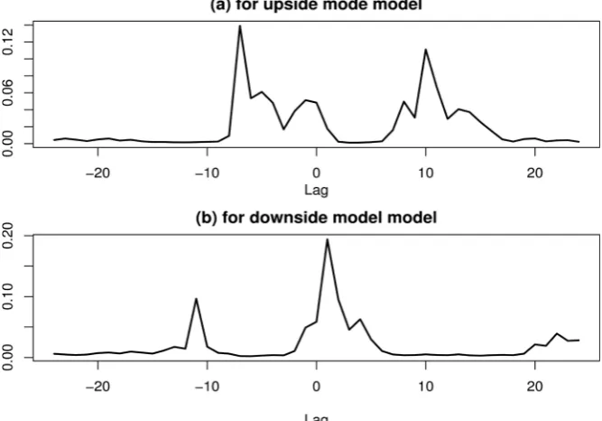
Figure 5 shows the relative likelihood distribution of the lags between −24 and 24 in the CPI models, with the units on the horizontal axis representing months. It can be seen from Figure 5 that two peaks exist in the panel showing the upside-mode model. Specifically, the left and right peaks correspond to around a seven-month lead and a 10-month lag. Therefore, the lead-lag relationship between GDP and the CPI is complicated during the expansion phase, where CPI movements sometimes lead those of GDP by seven months, while at other times they lag by 10 months. In other words, sometimes the CPI leads business expansion by about half a year, and sometimes it lags business expansion by about a year. Moreover, from the results for the downside-mode model, it can be seen that a higher peak in the relative likelihood is observed at around a lag of one month and a lower peak is seen at around a lead of 11 months. This implies that movements in the CPI almost coincide with movements in GDP, and sometimes lead CPI by about one year during the recession phase.

[image:10.595.207.541.469.702.2]

Figure 6 shows time series estimates for the time-varying coefficient in the upside-mode CPI models with (a) L1= −7 and (b) L1=10. It can be seen that when CPI movements lead GDP movements with L1= −7, the time-varying coefficient shows significantly negative values from 1990 to around 2000. This implies that the CPI had a negative effect on GDP from the time of the collapse of the bubble economy in Japan. However, when CPI movements lag GDP movements with L1=10, the time-varying coefficient is positive and the

(11)

[image:11.595.208.540.67.298.2]

[image:11.595.207.541.323.562.2]

Figure 6. Time series of the time-varying coefficient for upside-mode CPI models.

Figure 7. Time series of the time-varying coefficient for downside-mode CPI models.

absolute values have continued to rise. This implies that sometimes there are positive effects of GDP on CPI and such effects become stronger.

(12)

5. Conclusions

To analyze the relationship between economic growth and inflation in Japan, we proposed a Bayesian dynamic linear modeling method and used it to analyze the dynamic relationship between quarterly GDP data and monthly CPI data in Japan. First, we extracted stationary components from GDP and CPI time series using a set of state space models. Then, we constructed a set of Bayesian regression models with a time-varying coefficient. These models are two-mode regression with time-varying coefficient (TMR-TVC) models.

It should be emphasized that there are two important parameters in the TMR-TVC models: the time lag between GDP and the CPI and the time-varying coefficient. From the value of the lag, we can determine the lead-lag relationship, while from the estimate of the time-varying coefficient, we can analyze the dynamic relationship between GDP and the CPI.

Finally, using an empirical study based on the proposed method, we analyzed the dynamic relationship between the stationary components of GDP and the CPI using Japanese economic statistics from 1980 to 2005. The empirical study produced the following results. 1) The lead-lag relationship between GDP and the CPI is complicated. 2) The CPI had a negative effect on GDP from the time of the collapse of the bubble economy in Japan, and sometimes there are positive effects of GDP on the CPI in which the effects become stronger during the expansion phase. 3) GDP has a negative effect on the CPI, and this effect becomes stronger in periods of recession.

Acknowledgements

This work is supported in part by a Grant-in-Aid for Scientific Research (C) (16K03591) from the Japan Society for the Promotion of Science. We thank Geoff Whyte, MBA, from Edanz Group (www.edanzediting.com/ac) for editing a draft of this manuscript.

References

[1] Faria, J.R. and Carneiro, F.G. (2001) Does High Inflation Affect Growth in the Long and Short-Run? Journal of Applied Economics, 4, 89-105.

[2] Mallik, G. and Chowdhury, A. (2001) Inflation and Economic Growth: Evidence from South Asian Countries. Asian Pacific Development Journal, 8, 123-135. [3] Sweidan, O.D. (2004) Does Inflation Harm Economic Growth in Jordan? An

Aco-nometric Analysis for the Period 1970-2000. International Journal of Applied Eco-nometrics and Quantitative Studies, 1, 41-66.

[4] Mubarik, Y.A. (2005) Inflation and Growth: An Estimate of the Threshold Level of Inflation in Pakistan. State Bank of Pakistan—Research Bulletin, 1, 35-44.

[5] Erbaykal, E. and Okuyan, H.A. (2008) Does Inflation Depress Economic Growth? Evidence from Turkey. International Research Journal of Finance and Economics, 17, 1450-2887.

(13)

https://doi.org/10.1355/ae26-2d

[7] Jiang, X.-Q. (Kyo, K.) and Kitagawa, G. (1993) A Time Varying Coefficient Vector AR Modeling of Nonstationary Covariance Time Series. Signal Processing, 33, 315-331. https://doi.org/10.1016/0165-1684(93)90129-X

[8] Jiang, X-Q. (Kyo, K.) (1995) A Bayesian Method for the Dynamic Regression Analy-sis. Transactions of the Institute of Systems, Control and Information Engineers, 8, 8-16. https://doi.org/10.5687/iscie.8.8

[9] Kyo, K. and Noda, H. (2011) A New Algorithm for Estimating the Parameters in Seasonal Adjustment Models with a Cyclical Component. ICIC Express Letters: An International Journal of Research and Surveys, 5, 1731-1737.

[10]Kyo, K. and Noda, H. (2013) Bayesian Analysis of the Dynamic Relationship be-tween Oil Price Fluctuations and Industrial Production Performance in Japan. In-formation: An International Interdisciplinary Journal, 16, 4639-4660.

[11]Kyo, K. and Noda, H. (2015) Dynamic Effects of Oil Price Fluctuations on Business Cycle and Unemployment Rate in Japan. International Journal of Innovation, Man-agement and Technology, 6, 374-377.

[12]Kitagawa, G. (2010) Introduction to Time Series Modeling. CRC Press.