ISSN Online: 2169-2688 ISSN Print: 2169-267X
DOI: 10.4236/ars.2017.64019 Dec. 29, 2017 260 Advances in Remote Sensing
Salt-Affected Soil Mapping in an Arid
Environment Using Semi-Empirical
Model and Landsat-OLI Data
Abderrazak Bannari
1*, Ali El-Battay
1, Nadir Hameid
1, Fadia Tashtoush
21Department of Geoinformatics, College of Graduate Studies, Arabian Gulf University, Manama, Kingdom of Bahrain
2Department of Natural Resources and Environment, Arabian Gulf University, Manama, Kingdom of Bahrain
Abstract
The aim of this research is to map the salt-affected soil in an arid environment using an advanced semi-empirical predictive model, Operational Land Imager (OLI) data, a digital elevation model (DEM), field soil sampling, and labora-tory and statistical analyses. To achieve our objectives, the OLI data were at-mospherically corrected, radiometric sensor drift was calibrated, and distor-tions of topography and geometry were corrected using a DEM. Then, the soil salinity map was derived using a semi-empirical predictive model based on the Soil Salinity and Sodicity Index-2 (SSSI-2). The vegetation cover map was extracted from the Transformed Difference Vegetation Index (TDVI). In ad-dition, accurate DEM of 5-m pixels was used to derive topographic attributes (elevation and slope). Visual comparisons and statistical validation of the semi-empirical model using ground truth were undertaken in order to test its capability in an arid environment for moderate and strong salinity mapping. To accomplish this step, fieldwork was organized and 120 soil samples were collected with various degrees of salinity, including non-saline soil samples. Each one was automatically labeled using a digital camera and an accurate global positioning system (GPS) survey (σ ≤ ± 30 cm) connected in real time to the geographic information system (GIS) database. Subsequently, in the la-boratory, the major exchangeable cations (Ca2+, Mg2+, Na+, K+, Cl− and
2 4
SO −), pH and the electrical conductivity (EC-Lab) were extracted from a sa-turated soil paste, as well as the sodium adsorption ratio (SAR) being calcu-lated. The EC-Lab, which is generally accepted as the most effective method for
soil salinity quantification was used for statistical analysis and validation pur-poses. The obtained results demonstrated a very good conformity between the derived soil salinity map from OLI data and the ground truth, highlighting six major salinity classes: Extreme, very high, high, moderate, low and non-saline. How to cite this paper: Bannari, A.,
El-Battay, A., Hameid, N. and Tashtoush, F. (2017) Salt-Affected Soil Mapping in an Arid Environment Using Semi-Empirical Model and Landsat-OLI Data. Advances in Remote Sensing, 6, 260-291.
https://doi.org/10.4236/ars.2017.64019
Received: September 25, 2017 Accepted: December 26, 2017 Published: December 29, 2017
Copyright © 2017 by authors and Scientific Research Publishing Inc. This work is licensed under the Creative Commons Attribution International License (CC BY 4.0).
http://creativecommons.org/licenses/by/4.0/
DOI: 10.4236/ars.2017.64019 261 Advances in Remote Sensing The laboratory chemical analyses corroborate these results. Furthermore, the semi-empirical predictive model provides good global results in comparison to the ground truth and laboratory analysis (EC-Lab), with correlation
coeffi-cient (R2) of 0.97, an index of agreement (D) of 0.84 (p < 0.05), and low
over-all root mean square error (RMSE) of 11%. Moreover, we found that topo-graphic attributes have a substantial impact on the spatial distribution of sa-linity. The areas at a relatively high altitude and with hard bedrock are less susceptible to salinity, while areas at a low altitude and slope (≤2%) composed of Quaternary soil are prone to it. In these low areas, the water table is very close to the surface (≤1 m), and the absence of an adequate drainage net-work contributes significantly to waterlogging. Consequently, the intrusion and emergence of seawater at the surface, coupled with high temperature and high evaporation rates, contribute extensively to the soil salinity in the study area.
Keywords
Soil Salinity, Remote Sensing, Landsat-OLI, GIS, Semi-Empirical Model, Salinity Spectral Indices, Topographic Attributes, Arid Environment
1. Introduction
DOI: 10.4236/ars.2017.64019 262 Advances in Remote Sensing The measurement of electrical conductivity (EC) of saturation extract from a saturated soil paste is considered a standard and universally accepted way of measuring soil salinity [8][9]. Nevertheless, the cost of such salinity determina-tion becomes prohibitive when it calls for regular monitoring over a long period. These methods are expensive, time consuming, and require manpower to ac-complish this task. In addition, the dynamic nature of soil salinity in space and time makes it very difficult to use conventional methods for comparisons over large areas [10]. According to Metternicht and Zinck [6], remote sensing and GIS offer advantages over ground-based methods because they make it possible to map accurately vast areas that are subject to soil salinity hazards spatially and temporally with good accuracy. In the literature, various authors have examined the advantages of remote sensing methods and sensors for the assessment of sa-linity-based soil degradation [6] [7] [11]-[25]. Remote sensing methods can be relatively easy to use and reliable for these purposes. Their main advantage is that they enable mapping of large areas at a relatively low cost [26][27]. Infor-mation can also be collected at regular intervals, therefore making monitoring easier and less expensive. This not only allows for appropriate remedial action to be taken, but also to monitor both the effectiveness of any ongoing remediation or preventative measures that facilitate management and decision-making. Cur-rently, the most used source of imagery for salinity detection remains multispec-tral remote sensing with the Landsat series sensors [28][29][30][31][32].
Furthermore, some scientists have advocated the hypothesis that soil-salt oc-curs in many landscapes in response to the way water moves through and over the landscape. Indeed, terrain attributes contribute significantly to the flow paths and, therefore, to the soil salinity attributes [3][33]. Topography is recognized as an important factor in determining the stream flow response. It defines the effects of gravity on the movement of water in a watershed, and therefore it in-fluences many aspects of the hydrologic system [34]. Consequently, topographic attributes must be considered for the detection and mapping of soil salinity pa-rameters [35][36]. Morre et al.[37] have discussed the relationship between to-pographic attributes and hydro-geological processes in the landscape with regard to the salinity of a soil. Sheng et al.[38] integrated GIS environment climate va-riables, vegetation data, and topographic and geomorphologic features for salt-affected soil analysis mapping in China. Over Canadian territory, Florinsky
DOI: 10.4236/ars.2017.64019 263 Advances in Remote Sensing soils. According to McBratney et al.[36], the first requirement in soil characte-ristic mapping and soil salinity parameter detection is the integration of topo-graphic variables and ancillary data in the analysis. Bilgili [41] investigated the synergy between geomorphometry and remote sensing science for soil salinity mapping. In irrigated agricultural arid land, Elmahdy and Mohamed [42] hig-hlighted a strong correlation between flow accumulation, groundwater salinity, topographic attributes and salt-affected soil. In addition, they showed that the integration of remote sensing and GIS could be used in predicting and identify-ing sites of groundwater salinity in arid regions. In central Iran, Taghiza-deh-Mehrjardi et al. [31] demonstrated the potential of multispectral remote sensing data, EC, terrain parameters, and geomorphologic integration for soil salinity detection and mapping. The main objective of this research is to perform salt-affected soil mapping in an arid environment using a semi-empirical predic-tive model, Landsat-8 Operational Land Imager (OLI) data, a digital elevation model (DEM) for image topographic rectification and results interpretation, field soil sampling, and laboratory and statistical analyses. In comparison with stochastic and integrated approaches [1][43], its originality resides in its sim-plicity and rapidity in developing and integrating an operational methodology for slight, moderate and strong salinity mapping on the regional scale in an arid environment.
2. Materials and Methods
The used methodology in this research is summarized in four steps. Firstly, the preprocessing step involves the OLI image corrections from the atmosphere, the radiometric drift of the sensor, and the topographic and the geometric distor-tions using a high spatial resolution (5-m) DEM. Secondly, the processing step addresses the soil-salinity map retrieval using an advanced semi-empirical model for salinity detection based on the Soil Salinity and Sodicity Index-2 (SSSI-2). In addition, vegetation cover was extracted based on the Transformed Difference Vegetation Index (TDVI) using EASI-modeling of PCI-Geomatica [44]. The to-pographic variables of elevation and slope were obtained using a DEM in the ArcGIS environment [45]. Thirdly, for statistical analysis and validation pur-poses, fieldwork was organized and 120 soil samples were collected with various degrees of salinity, as well as non-saline soil samples. Each sample was automat-ically labeled using a digital camera and accurate global positioning system (GPS) survey (σ ≤ ±30 cm) connected in real time to the GIS database. Then, it was analyzed in the laboratory to extract electrical conductivity (EC-Lab) from a
saturated soil paste, which is generally accepted as the most effective method for soil salinity quantification. In addition, the major exchangeable cations (Ca2+,
Mg2+, Na+, K+, Cl− and 2 4
DOI: 10.4236/ars.2017.64019 264 Advances in Remote Sensing (EC-Lab), spatial distribution of vegetation cover, ancillary data (soil, geology and
geomorphology maps) and topographic attributes.
2.1. Study Site
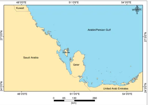
The Kingdom of Bahrain (26˚00'N, 50˚33'E) is a group of islands located in the Arabian Gulf, east of Saudi Arabia and west of Qatar (Figure 1). The archipelago comprises 33 islands, with a total land area of about 765.30 km2[46]. According
[image:5.595.61.538.307.646.2]to the aridity criteria and the great variations in climatic conditions, Bahrain has an arid to extremely arid environment [47]. High summer temperatures of around 45˚C (June-September) and an average of 17˚C approximately charac-terize the main island in winter (December-March). Rain is sparse, and occurs primarily from November to April, with an annual average of 72 mm, sufficient only to support the most drought-resistant desert vegetation. Mean annual rela-tive humidity is over 70% due to the surrounding Arabian Gulf waters, and the annual average potential evapotranspiration rate is 2099 mm [48].
Figure 1. Study site (Kingdom of Bahrain).
DOI: 10.4236/ars.2017.64019 265 Advances in Remote Sensing marls and shales. The leading structure is the north-south axis of the main dome, with minor cross folds predominantly tilting from northeast to southwest. The beds are gently inclined towards the coast from the center of the main isl-and. The fringes of Bahrain are covered by more recent marine and Aeolian sand dunes, which were derived from the Arabian land connection across the present Arabian Gulf [49].
2.2. OLI Landsat-8 Data
Since 1972, the Landsat satellite program, involving NASA, the USGS and other agencies, has provided a continuous record of the Earth’s surface reflectivity from space. Indeed, the Landsat satellites series supports more than four decades of global moderate resolution data collection, distribution and archives of the Earth’s surface [50] to support research, applications, and climate change impact analysis on a global, regional and local scale. With the Landsat-5 satellite trans-mitting its final image in early 2013, and with Landsat-7 still in orbit, but com-promised by Scan Line Corrector problems since 2003, the continuity of the Landsat program was ensured with the launch of Landsat-8 in February 2013 with the OLI instrument on board. Its design results in a more sensitive instru-ment, providing improved land-surface reflectivity and information extraction with far fewer moving parts. With a significant amelioration of the sig-nal-to-noise ratio (SNR) radiometric performance quantized over a 12-bit dy-namic range (Level 1 data), products are delivered in 16 bit compared to pre-vious Landsat sensors (TM and ETM+) using only 8 bit [51]. This SNR perfor-mance and improved radiometric resolution provide a superior dynamic range and reduce saturation problems associated with maximizing the range of land-surface spectral radiance and, consequently, enable better characterization of land-cover conditions [52]. The OLI image used in this research was acquired on April 5, 2015 and was deemed acceptable in terms of cloud cover and spatial coverage of the study area.
2.3. OLI Data Preprocessing
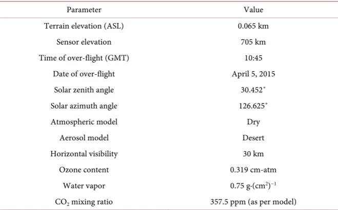
DOI: 10.4236/ars.2017.64019 266 Advances in Remote Sensing coefficients (gain and offset) in the image metadata file for deriving apparent ra-diance or apparent reflectance values from the OLI sensor data. Furthermore, two processes that are responsible for the modification of the satellite signal— mainly absorption by gases (ozone, water vapor, and carbon dioxide) and scat-tering by aerosols and molecules [62]-dominate atmospheric effects. These phe-nomena cause an attenuation of the signal in the direction of illumination, but increase the signal in the other directions causing a scattering effect. An accurate correction of atmospheric effects requires a priori knowledge of the atmospheric parameters that interfere with image data acquisition. For our image, these pa-rameters were measured during the satellite overpass using meteorological sta-tion data located at the closest point to the study site. The Canadian Modified Simulation of the Satellite Signal in the Solar Spectrum (CAM5S), based on the Herman radiative transfer code [63], was used for atmospheric parameter simu-lation in this study. CAM5S simulates the signal measured at the TOA from the Earth’s surface reflecting solar and sky irradiance at sea level, while considering the OLI sensor characteristics, such as the band passes of the solar-reflective spectral bands (Figure 2), satellite altitude, atmospheric condition, atmospheric model, Sun and sensor geometry, and terrain elevation. Consequently, all the requested atmospheric correction parameters were used to transform the ap-parent reflectance at the TOA to the ground reflectance, ρG(λ), using Equation
(3). Table 1 summarizes the input parameters for the CAM5S radiative transfer code (RTC). To preserve the radiometric integrity of our image, absolute radi-ometric calibration and atmospheric effects (scattering and absorption) were combined and corrected in one-step [64] as follows:
( )
( )
( )
( )
*
L
λ
=Gλ
DNλ
+Oλ
(1)( )
( )
( )
( )
* * 2
0 cos s
L D E
ρ λ =π⋅ λ ⋅ λ ⋅ θ (2)
( )
( )
( )
( )
( )
( )
( )
* 1 s v a G G T T tg S θ θ λ λρ λ λ ρ λ ρ λ
ρ λ ⋅ = ⋅ + ⋅ − ⋅
(3)
where:
( )
*
L
λ
= Apparent equivalent spectral radiance at TOA [Watts. (m2 sr μm)−1],( )
G
λ
= Radiance multiplicative rescaling factor from the metadata (gain),( )
O
λ
= Radiance additive rescaling factor from the metadata (offset),( )
DN
λ
= Digital number values,( )
0
E
λ
= Irradiance [Watts. (m2 sr μm)−1],D
= Earth-Sun distance [astronomical units],( )
*
ρ λ
= Apparent reflectance at the TOA, with a correction for solar zenith angle,( )
aρ λ
= Atmospheric at-sensor reflectance,( )
Gρ λ
= Ground reflectance,( )
tg
λ
= Average total gaseous transmittance,( )
sDOI: 10.4236/ars.2017.64019 267 Advances in Remote Sensing
( )
vT λ θ = Total ascending scattering transmittance, and
s
θ = Solar zenith angle,
v
θ = Sensor zenith angle,
[image:8.595.61.537.72.398.2]S = Spherical albedo.
Figure 2. Relative response profile of the OLI Landsat-8 sensor and atmospheric transmittance.
Table 1. Input parameters for the CAM5S RTC (ASL: Above sea level; GMT: Greenwich Mean Time; ppm: Parts per million).
Parameter Value
Terrain elevation (ASL) 0.065 km
Sensor elevation 705 km
Time of over-flight (GMT) 10:45
Date of over-flight April 5, 2015
Solar zenith angle 30.452˚
Solar azimuth angle 126.625˚
Atmospheric model Dry
Aerosol model Desert
Horizontal visibility 30 km
Ozone content 0.319 cm-atm
Water vapor 0.75 g·(cm2)−1
CO2 mixing ratio 357.5 ppm (as per model)
2.3.2. Geometric and Topographic Corrections
[image:8.595.208.538.460.665.2]DOI: 10.4236/ars.2017.64019 268 Advances in Remote Sensing alignment knowledge, refining the alignment of the sub-images from the mul-tiple OLI sensor chips, and refining the spatial alignment of the OLI spectral bands. The results showed that the considered aspects of geometric performance met the system accuracy requirements [65]. However, one of the remote sensing objectives is to provide quantitative information for producing conform and standard cartographic documents and deriving digital data files compatible with GIS databases. Within this framework, rigorous geometric and topographic cor-rections of satellite image data are essential for digital analyses and for use with GPS and GIS databases [66]. The Landsat-OLI data as delivered from the USGS EROS Center were geometrically corrected and registered to the WGS-84 geo-detic reference. However, even a second-degree polynomial function cannot eliminate all the distortions caused by terrain relief and shadow. Indeed, the in-tersection of the FOV sensor with the terrain altitude variation may well produce pixels with variable size following the slope and aspect (moderately negligible for OLI due to its relatively narrow FOV), and varying spectral signature from uni-form and similar targets. Accordingly, the association of topographic variation with illumination geometry [67] can result in considerable spectral signature variation for a given target. For correcting terrain relief effects, it is necessary to have an altitude value for each point in the image. This is provided using a spa-tially co-registered DEM in which the sampling step of the DEM must be at the image pixel size or a higher spatial resolution to provide an ortho-image with good precision [66][68]. In this study, an ortho-rectification was conducted us-ing a highly accurate DEM with a 5-m pixel size [69][70], and processed using the Rational-Function model implemented in the Ortho-Engine module of PCI-Geomatica [44]. Topographic attributes, such as altitude, slope, aspect, and sky view were integrated into the ortho-rectification approach and extracted from the DEM [71]. This step enabled corrections of the parallax effect on the spatial arrangement of long-track pixels, as well as minimizing the disruptive ef-fects caused by shadow and topographic variability, and the residual atmospher-ic artefacts caused by altitude variability. Additionally, it allowed the integration of a derived salinity map into a GIS with GPS locations of soil sampling points for validation analysis. To preserve the image’s radiometric integrity, geometric corrections have been combined into a single step with the correction of topo-graphic effects [71] utilizing a set of equations in one processing data flow.
2.4. Predictive Model for Soil Salinity Mapping
DOI: 10.4236/ars.2017.64019 269 Advances in Remote Sensing environment using satellite and ground truth data. Using ground-based spectral data, Al-Khaier [75] developed the Salinity Index using bands 4 and 5 of the ASTER sensor (SI-ASTER) to derive agricultural soil salinity in semi-arid irri-gated agricultural regions of Syria. A cooperative project between India and the Netherlands [27] also proposed a methodology for soil salinity and waterlogging mapping in irrigated cropped land in a semi-arid region of India. They recom-mended three different Salinity Indices (SI-1, SI-2 and SI-3) using Landsat-TM Bands 4, 5 and 7. Bannari et al.[16] used ground spectroradiometric measure-ments and reflectance processing to simulate EO-1 ALI sensor spectral bands and demonstrated that the SWIR bands are more sensitive than other band-widths to different degrees of salinity and sodicity, especially for slight and moderate levels. They proposed two indices: Soils Salinity and Sodicity Indices 1
and 2 (SSSI-1 and SSSI-2), which are particularly well-suited for low and me-dium salinity identification. Furthermore, using spectroradiometric measure-ments and EC extracted from saturated paste, all of these nine spectral salinity indices discussed above were derived from the spectra. They were then corre-lated to EC using a second order regression analysis, at 90% confidence level, to establish a semi-empirical model for soil salinity detection [16]. A comparative study among these models for soil salinity detection in North Africa using ALI EO-1 imagery showed that the model based on SSSI-2 provided the most accu-rate information for soil salinity detection mapping [7] [24]. In this study, we therefore considered this predictive model:
(
)
2(
)
Predicted
EC- =Cst⋅4521 SSSI-2 +125 SSSI-2 +0.41 (4)
(
OLI-6 OLI-7 OLI-7 OLI-7) (
OLI-6)
SSSI-2=
ρ
⋅ρ
−ρ
⋅ρ
ρ
(5)where:
st
C : Scaling factor,
Predicted
EC- : Predicted EC from remote sensing semi-empirical model,
OLI-6
ρ : Reflectance in OLI SWIR-1 channel, and
OLI-7
ρ : Reflectance in OLI SWIR-2 channel. The scaling factor ( st
C ) enables an up-scaling between the spatial information
measured in the field (fine scale) and its homologous information derived from the image (coarse scale). In the literature, several methods exist to calculate this factor depending on the remote sensing applications [19]. In this research, a simple up-scaling empirical ratio was calculated between the observed and the predicted values considering five sampled points representing the five salinity classes (extreme, very high, high, moderate, low and non-saline). Homogeneous and uniform pixel surface representing each class was located using the GPS coordinates; their homologous ground reference values resulting from the labor-atory analysis (EC-Lab) were used to calculate five scaling factor values. An
aver-age value was then calculated as a global scaling factor for the entire imaver-age.
2.5. Vegetation Cover Mapping
prod-DOI: 10.4236/ars.2017.64019 270 Advances in Remote Sensing uctivity. However, diverse halophytic plants grow in an arid environment ac-cording to their tolerance to salinity and the alkalinity of the soil [74]. Therefore, vegetation cover can be used to assess the spatial variability degree of soil salini-ty. The monitoring of vegetation cover involves the utilization of vegetation in-dices as a spectro-radiometric measurement of spatial and temporal patterns of vegetation photosynthetic activity. In the literature, over fifty vegetation indices have been developed to measure the vegetation cover in different applications and under quite particular conditions, as reviewed by Bannari et al. [76]. How-ever, various physical effects on the signal at the sensor can limit the use of these indices to characterize vegetation cover. These include drift of the sensor radi-ometric calibration, atmospheric variations, topographical distortions, optical soil properties artifacts, bi-directional effects, spatial and spectral characteristics of the sensors, and problems of saturation and linearity [7][56][77][78] [79]. These factors increase or decrease reflectances in the red and NIR spectral bands and, consequently, limit the detection of vegetation cover changes using vegeta-tion indices, causing errors in the modeling process. The majority of these prob-lems can be corrected for remote sensing imagery or in situ measurements be-fore the derivation of vegetation indices. However, the problems of the satura-tion and linearity and soils’ background artifacts, especially in arid and semi-arid environments where the vegetation cover is not dense, are the weaknesses that result from the design and the analytical formulation of the vegetation indices. To deal with the saturation, the linearity weaknesses, and the soils artefacts effect correction, the TDVI was developed [80] to describe the dynamic range of the vegetation-soil systems linearly and independently of optical soil proprieties in different applications using remotely sensed data. This TDVI index was derived using EASI-modeling in PCI-Geomatica [44] and used in this study to analyze the impact of salinity on the spatial distribution of vegetation cover over the study site.
(
)
2OLI-5 OLI-4 OLI-5 OLI-4
TDVI 1.5= ρ −ρ ρ +ρ +0.5 (6)
where:
OLI-4
ρ = Reflectance in OLI red channel, and
OLI-5
ρ = Reflectance in OLI near-infrared channel.
2.6. Soil Sampling and Laboratory Analyses for Validation
DOI: 10.4236/ars.2017.64019 271 Advances in Remote Sensing preferred, but logistical and financial constraints often preclude its use, especial-ly over large territories [9]. Indeed, in practice it is not logistically realistic or economically possible to measure the EC uniformly and densely over the King-dom of Bahrain. To overcome this situation, 120 soil samples were selected based on the spatial representativeness of the major soil classes and various de-grees of salinity.
The soils of Bahrain are characterized by five different soil classes of moderate to shallow depth, and are closely related to the geology and geomorphology of the terrain [49]. We distinguish between two classes of Solonchak soils. Note that the term “Solonchak” soil class has been used to present salty soils where a capillary rise of solutions containing soluble salts occur [83]. The natural Solon-chak refers to soils with no agricultural activities and which retain a high gyp-sum content (very high and with high salinity). Moreover, there is the cultivated Solonchak soil class, which is located in areas with current or previous agricul-tural activities. The Regosols soil class with moderate salinity is depicted as a mixture of raw mineral, similar to the natural Solonchak soils, with the possibil-ity for growing scattered halophytic plants. The miscellaneous land class catego-ry that is a composition of silts and fine sands with a low level of salinity. This class is acceptable for agriculture, is very limited and is situated in zones of rela-tively low altitude and slope. Finally, the non-saline soil class, which is imported to build artificial islands.
Soil sample collection was carried out between 2 and 7 April, 2016. The Ba-hrain soil map was used as a reference for the sampling data, and 120 samples were selected based on the spatial representativeness of the major soil classes as discussed above and by considering various degrees of salinity and the non-saline soil. Samples were taken from the upper layer (5 cm deep) of the soil, in an area of about 50 × 50 cm2. Observations and remarks about each sample
(color, brightness, texture, etc.) were noted. The location of each point was au-tomatically labeled and recorded using a 35 mm digital camera equipped with a 28 mm lens and accurate GPS survey (σ ≤ ±30 cm) connected in real time to the GIS database. Then, each sample was analyzed in the laboratory in order to ex-tract the major exchangeable cations (Ca2+, Mg2+, Na+, K+, Cl− and 2
4 SO −), the EC-Lab, pH, and the SAR from a saturated soil paste. These elements were
ana-lyzed using methods that meet the current international standards in soil science [84]. Because the electrical conductivity is considered an accurate measure of soil salinity [8], the derived values in the lab (EC-Lab) for all sampling points were
overlaid on the remote sensing predictive salinity map (EC-Predicted) in a GIS
en-vironment in order to obtain spatial correspondences between sampling points and their homologous pixels, for validation purposes. The statistical analysis was conducted by correlating those values (EC-Lab and EC-Predicted) using linear
regres-sion at the significance level p < 0.05.
2.7. Statistical Analyses
DOI: 10.4236/ars.2017.64019 272 Advances in Remote Sensing were calculated for both EC ground sampling points obtained from the laboratory analysis (EC-Lab) and the predicted values derived from OLI data (EC-Predicted)
us-ing the semi-empirical model. Standard deviation statistics enabled the evalua-tion of data variability. This parameter was reported in all cases as an error per-centage of the average values extracted from the ground sampling point (ECG-Lab)
and image data (EC-Predicted). For validation purposes, EC-Lab and EC-Predicted were
compared using the 1:1 line. Ideally, observed and predicted values should have a correspondence of 1:1. The index of agreement D reflects the degree to which the observed value is accurately estimated by the predicted value. This measure was calculated as follows [85]:
(
)
(
)
2 1 2 1 1 n i i i n i i i P O D P O = = − = − ′+ ′ ∑
∑
(7)where Pi is the predicted value at sample i, Oi is the observed value at sample i,
i
P′ is the difference between Pi and the average of the predicted values, and Oi′
is the difference between Oiand the average of the observed values and n is the
number of values. This index provides a measure of the degree to which a mod-el’s predictions are error-free. The index ranges between 0 and 1, with 1 indicat-ing a perfect match between observed and predicted values. The observed values were those calculated from each sampling point at the laboratory (EC-Lab) and
the predicted values were from the salt-affected soil map using the semi-empirical model and OLI image (EC-Predicted). The root mean square error (RMSE) was used
as an overall error to supplement the index of agreement described above. This error also quantifies the 1:1 relationship between observed and predicted values. It was calculated as follows [85]:
(
)
21 RMSE n i i i P O n = −
=
∑
(8)The relationships between observed and predicted values were also analyzed using a linear regression model. The correlation coefficient (R2) of the regression
model was also used to evaluate the strength of the linear relationship between observed (EC-Lab) and predicted values (EC-Predicted). Systematic linear
overpre-dictions or underpreoverpre-dictions generate characteristic variations in the slope and intercept values, which can help to interpret the major sources of error and the potential of the semi-empirical model for salinity mapping and prediction using OLI data.
3. Results and Discussion
3.1. Visual Assessment and Statistical Analysis of Soil
Salinity Maps
DOI: 10.4236/ars.2017.64019 273 Advances in Remote Sensing accuracy directly to our field observations, laboratory analyses, and statistical va-lidation. Globally, the results show that the semi-empirical model based on the SSSI-2 index provided a satisfactory result in comparison to the ground truth, laboratory analyses, as well as good agreement with spatial distribution of vege-tation cover derived with TDVI index, ancillary data (soils, geology, and geo-morphology maps), and topographic attributes.
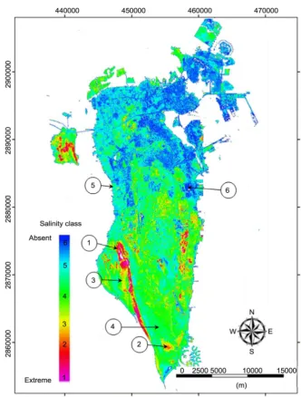
Figure 3. Soil salinity map derived using the predictive model based on SSSI-2 index, highlighting six major salinity classes: extreme (class 1), very high (class 2), high (class 3), moderate (class 4), low (class 5), and non-saline (class 6).
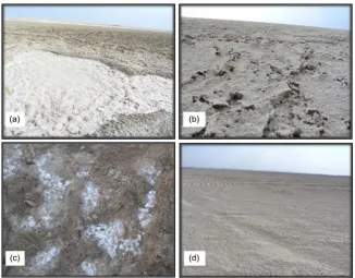
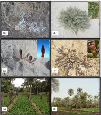
DOI: 10.4236/ars.2017.64019 274 Advances in Remote Sensing (class 6 in dark blue). The visual analysis and validation of these classes by ref-erence to the field visit (ground truth) reveals a good conformity. The extreme salinity class is characterized by the presence of high contents of soluble salts and the surface salt crust (Figure 4(a)). This class depicts the sabkha position reliably based on our GPS field locations. These sabkha zones create a chemically aggressive environment and lead to a structurally unstable soil condition. They are natural solonchaks and are uncultivated (loamy and sandy, highly gypsifer-ous) and devoid of any vegetation. Sulfates, chlorides and carbonates of sodium, calcium and magnesium dominate the salt content in this sabkha soil. Seawater intrusion and subsequent evaporation results in surface crusts, especially in these zones of capillary rise, where the terrain elevation is less than a few centimetres above mean sea level (very close to ground surface), and where the slope is near zero, thus facilitating water catchment and retention. This situation generally occurs in a dry climate, such as the case of Middle Eastern countries, where the temperature is very high, the rainfall is insufficient to leach salts and excess so-dium ions out of the soil, and high evaporation rates accelerate the salt accumu-lation and its concentration at the soil surface.
Figure 4. Extreme salinity class (a), very high saline class (b), high saline class (c), and moderate saline class (d).
DOI: 10.4236/ars.2017.64019 275 Advances in Remote Sensing with cementation increasing with depth. The layering is characterized by alter-nating shell-rich and shell-poor layers. The material of this area is a mixture of medium and fine sand-grade quartz with moderate amounts of carbonate. The soil surface (~5 cm) becomes cemented, forming a strong, white-brown crust of salt. In other places, the immediate top surface becomes indurated into a brittle crust, which is ridged into many undulations with an amplitude of 3 to 5 cm. Moreover, similar to the two previously described classes, the areas of this class are completely devoid of vegetation, as illustrated by the field photos (Figure 4). The moderate saline class (class 4, green color in Figure 3) illustrates the domi-nant class in the southern half of Bahrain island (Figure 4(c)). The soils are moderate to shallow in depth, calcareous to highly calcareous, with calcium car-bonate equivalents ranging from 15% - 30% and dominated by shells and sand with fine contents varying from 5% to 30 %. They contain moderate amounts of gypsum, mainly in the upper 75 cm of the soil profile [49]. The soils of this class are characterized by very poor organic matter content, and are not suitable for agricultural production. However, very sparse and scattered clumps of halo-phytic (salt tolerant) plants are observed in this class area (Figures 5(a)-(d)). For instance, we found the “zygophyllum simplex” (Figure 5(a)), which is a de-licate plant with subsessile to very short petiolate leaves. The “Suaeda vermicu-lata Forssk” (Figure 5(b)) is a perennial herb, forming huge bushes or shrubs, usually with thicker leaves varying from cylindrical to thick and flattened, which support a high temperature and growth in saline soil. Moreover, there is the “cynomorium coccineum L.” (Figure 5(c)), which grows easily in the desert, particularly in sandy places. This plant has no chlorophyll and is unable to pho-tosynthesize. It is a geophyte, spending most of its life underground, and is a salt-tolerant plant. In addition, we found the “Halopeplis perfoliata” (Figure 5(d)) which is green to brownish in color, has low and woody branches with leaves that encircle the branches as swollen beads, and tolerates saline conditions [86].
According to the field visit and ancillary data (soil, geological and geomor-phological maps), we find that these first four saline classes (extreme, very high, high and moderate) are globally characterized by Eocene, Neocene and Miocene rocks. They are partly covered by Quaternary sediments and a complex of Pleis-tocene deposits that are often rich in calcium sulfate and sodium chloride and associated with shales and marls, limestone and dolomitic-limestone. Their gypso-saline characteristics cause the formation of salt strata that are thrust up-ward to the surface from the underlying salt bed. These saline formations are of-ten associated with anhydrite, gypsum, sulfur, and paleo-lagoonary sedimentary rocks.
DOI: 10.4236/ars.2017.64019 276 Advances in Remote Sensing 5 parts per million (ppm) in the saturation extract of the topsoil. Phosphorus availability is relatively low and this is commonly associated with highly calca-reous soils (P-fixation). The available phosphorus content is very much variable (3 - 50 ppm), and the available potassium content ranges from 100 - 360 ppm, as demonstrated by Al-Shabaani [87]. These class zones are the only cultivated areas in Bahrain and their extent is about 6000 ha (8% of the total area of the country), of which about 95% is equipped with irrigation systems. These areas are mainly used for growing date palms, alfalfa, vegetables and fodder crops, as illustrated in Figure 5(e) and Figure 5(f). According to the last agricultural census [88], this agricultural area decreased from 36.96% in 1995 to 33.89% in 1997 due to the salinity of irrigation water. Finally, the non-saline class (class 6, blue color in Figure 3) describes accurately the man-made (artificial) infra-structure, industrial and urban zones. This accurate visual discrimination analysis among different salinity classes demonstrates the robustness of the semi-empirical model used and its significant sensitivity to the complexity of salinity classes in this arid environment.
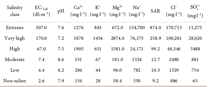
DOI: 10.4236/ars.2017.64019 277 Advances in Remote Sensing Likewise, the major exchangeable cations in the considered soil samples (Ca2+,
Mg2+, Na+, K+, Cl− and 2 4
SO −), pH, EC-Lab, and SAR values were determined in the laboratory from saturated soil paste extract (Table 2), and they corroborate the remote sensing results. Table 2 summarizes the average values of these chemical elements that are calculated from the sampling points representing each soil class separately. These analyses reveal a very high concentration of so-dium (Na+), which generally exceeds the sum of calcium (Ca2+) and magnesium
(Mg2+), and dominant chloride anion (Cl−) which exceeds sulfates ( 2 4 SO −). Moreover, we see that globally, the values of EC-Lab, Na+, and SAR increase
gradually and very significantly from non-saline soil to extreme soil salinity (sabkha). Indeed, the non-saline and low soil salinity classes (Miscellaneous soils), which support the agricultural system in Bahrain, are characterized by low EC (2.6 ≤ EC-Lab ≤ 4.4 dS·m−1) and SAR ≤ 10.3. The moderate salinity class
(EC-Lab ≈ 7.4 dS·m−1 and SAR ≈ 12.7) is the dominant soil class in Bahrain and is
a part of the Regosols soil category that allows for the growth of halophytic plants (Figures 5(a)-(d)). Contrariwise, the other three soil salinity classes with extreme, very high and high salinity content show very strong and extreme EC (67 ≤ EC-Lab ≤ 600 dS·m−1) and very high SAR (≥99.2) values. These three classes
[image:18.595.208.539.496.635.2]describe the natural Solonchak soil category. Obviously, these results are in agreement with the predicted salinity classes ascertained by remote sensing me-thod (Figure 3), and this is illustrated by the photographs acquired during the field visit (Figure 4) based on the GPS and GIS locations. Moreover, the pH values (7.1 to 8.6) are very informative as regards the preponderance of carbo-nate and the presence of bicarbocarbo-nate in the soils and, consequently, contribute significantly to the alkalinity aspect of the soil.
Table 2. Laboratory determination of EC-Lab, pH and ions content in the different soil
sa-linity classes.
Salinity
class (dS·mEC-Lab −1) pH Ca 2+
(mg·l−1) K +
(mg·l−1) Mg 2+
(mg·l−1) Na +
(mg·l−1) SAR Cl −
(mg·l−1) 2 4
SO−
(mg·l−1)
Extreme 507.0 7.6 1276 843 672.0 154,700 874.0 170,715 11,275 Very high 170.0 7.2 1878 1454 2874.0 76,373 258.9 100,281 28,020 High 67.0 7.5 1905 651 1581.0 24,171 99.2 48,546 5488
Moderate 7.4 8.6 531 67 181.0 1324 12.7 2480 881
Low 4.4 8.2 284 44 96.0 782 10.3 1329 754
Non-saline 2.6 7.9 154 28 58.4 530 9.2 886 63
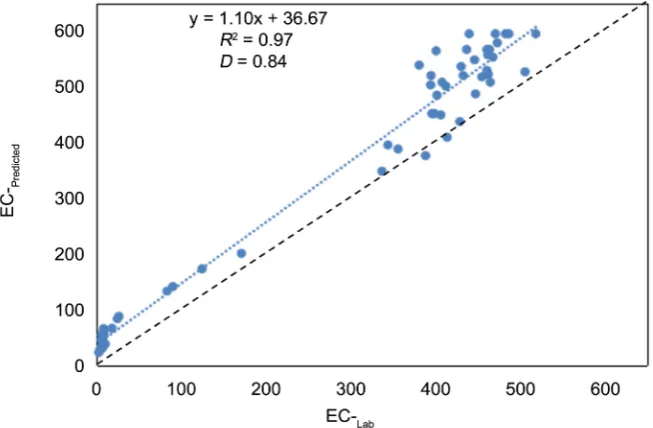
Figure 6 illustrates the relationship between the predicted electrical conduc-tivity values (EC-Predicted) derived from the OLI data and the ground reference
values resulting from the laboratory analysis (EC-Lab). Globally, the statistical
DOI: 10.4236/ars.2017.64019 278 Advances in Remote Sensing RMSE (11%). The scatter plot, as presented in Figure 6, reveals a good linear re-lationship between the two variables with a correlation coefficient (R2) of 0.97, at
significance level p < 0.05. The scatter plot, depicting the relationship between EC-Lab and EC-Predicted, illustrates a generally good fit to 1:1 line with an excellent
spatial variability of soil salinity (2.6 ≤ EC-Lab ≤ 600 dS·m−1). The classes with an
electrical conductivity of lower than 200 dS·m−1 are appropriately predicted by
the model, with an RMSE of around 5%. However, the electrical conductivity classes between 400 and 600 dS·m−1 were overestimated, resulting in the data not
fitting the 1:1 line very well. The slope and the intercept corroborate these ob-servations by expressing a slight deviation from the 1:1 line, with an RMSE of around 21%. This is likely because the model was developed for slight and mod-erate salinity in a semi-arid environment [7] and not for cases of extreme salinity in arid land. Moreover, scaling issues between the samples collected in the field representing an area of about 50 × 50 cm2 and its homologous points in the OLI
image, represented by a pixel (900 m2), may contribute to this slight variation. In
addition, the preprocessing of OLI data is essential and it will affect the integrity of the surface reflectance retrieval from the at-sensor radiance data. The sources of errors in the data preprocessing were reduced significantly by applying dif-ferent techniques for the removal of sensor artifacts and atmospheric effects. However, it is probable that residual errors persist (because we correct each spectral band uniformly and not pixel-by-pixel), causing a small difference be-tween the EC-Lab measured at the laboratory and their homologous EC-Predicted
[image:19.595.212.539.468.682.2]based on the remote sensing image. However, despite these small variations, the semi-empirical predictive model used provides satisfactory results in compari-son to the ground truth.
Figure 6. Relationship between electrical conductivity analyzed in the laboratory (EC-Lab
in dS·m−1) and the predicted values
(EC-Predicted in dS·m−1) derive from the semi-empirical
DOI: 10.4236/ars.2017.64019 279 Advances in Remote Sensing
3.2. Spatial Distribution of Vegetation Cover According to Soil
Salinity Classes
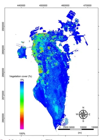
With reference to ground truth, the vegetation cover map derived using TDVI (Figure 7) illustrates an excellent agreement and relationship with the salinity map (Figure 3). Indeed, in the southern half of Bahrain island and the entire in-terior basin where salinity is present, the vegetation cover and agricultural activ-ities are completely absent. In addition, in the island’s northeast, where the in-frastructure is developed, the vegetation cover is deficient. Only the northwest areas show a relative vegetation cover, where the red color spots in the Figure 7 illustrate the date-palm clusters, while the dark and clear green colors show the agricultural fields (alfalfa, vegetables and fodder crops; see Figure 5(e) and Fig-ure 5(f)). In these vegetated areas, the soil salinity (2.6 ≤ EC-Lab ≤ 8 dS·m−1) is
highly heterogeneous from irrigated to non-irrigated sites depending on the quality of the groundwater used in irrigation. In fact, the agricultural lands are affected by saline water used for the irrigation preprocess. Additionally, the in-trusion of seawater, the shallow saline water table, the absence of an adequate drainage system and inappropriate soil-water management contribute signifi-cantly to the salinity of the agricultural lands. In addition to the low salinity in these areas, the soils also show sodic characteristics, since the soil structure is completely absent or poorly defined (dispersion and destruction of clay par-ticles). These results are in agreement with the soil chemical laboratory analysis, as discussed previously (pH between 7.1 and 8.6, see Table 2).
DOI: 10.4236/ars.2017.64019 280 Advances in Remote Sensing Figure 7. Derived vegetation map using TDVI.
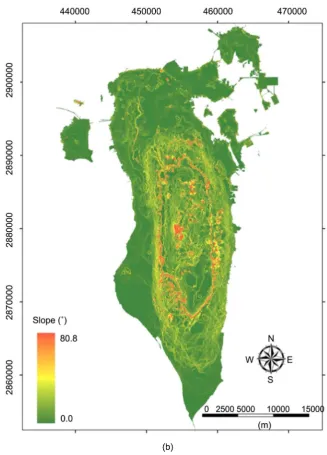
DOI: 10.4236/ars.2017.64019 281 Advances in Remote Sensing (Figure 8) are located on highly fractured carbonate rocks and coastal deposits, and are in accordance with those areas of high groundwater potential of variable salinity that occur close to or at the surface, as shown in our salinity map (Figure 3).
DOI: 10.4236/ars.2017.64019 282 Advances in Remote Sensing Figure 8. Elevation map (a) and slope map (b).
agree-DOI: 10.4236/ars.2017.64019 283 Advances in Remote Sensing ment with other scientists’ results elsewhere in the world [3] [89]-[94].
4. Conclusions
In this research, we carried out salt-affected soil mapping in an arid environ-ment using Landsat-OLI data, DEM, field soil sampling, a semi-empirical dictive model, and laboratory and statistical analyses. The OLI data were pre-processed from the atmosphere, the sensor radiometric drift, the geometric dis-tortions, and topographic variabilities. Then, the soil salinity map was derived using a semi-empirical predictive model based on the SSSI-2, as well as the ve-getation cover map being extracted from the TDVI. Moreover, topographic attributes were derived using accurate DEM of 5-m pixel in size. For statistical analysis and validation purposes, fieldwork was organized and 120 soil samples, as well as non-saline soil samples, were collected with various degrees of salinity. Each sample was automatically labeled using a digital camera and accurate GPS survey (σ ≤ ±30 cm) connected in real time to the GIS database, and was then analyzed in the laboratory both to measure the major exchangeable cations in the considered soil samples (Ca2+, Mg2+, Na+, K+, Cl− and 2
4
SO −), pH, EC-Lab, and to calculate the SAR from a saturated soil paste extract.
Globally, the visual validation step demonstrated a very good conformity be-tween the derived soil salinity map and the ground truth, highlighting six major salinity classes: extreme, very high, high, moderate, low and non-saline. It shows the efficacy of the semi-empirical model used to discriminate accurately among different and complex salinity classes, from sabkha to non-saline soils. The chemical laboratory analyses corroborate these remote sensing results and field observations. They reveal a very high concentration of sodium (Na+), which
generally exceeds the sum of Ca2+ and Mg2+, and dominant Cl− that exceed
2 4
SO − for the six salinity classes taken into consideration. Moreover, the values of EC-Lab, Na+, and SAR increased gradually and very significantly from the
non-saline soil to the extreme soil salinity (sabkha). Indeed, the non-saline and low soil salinity classes, which support the agricultural system in Bahrain, are characterized with low EC (2.6 ≤ EC-Lab ≤ 4.4 dS·m−1) and SAR (≤10.3). The
moderate salinity class with EC-Lab of around 7.4 dS·m−1 and SAR ≤ 12.7 is the
dominant soil class in Bahrain, allowing for the growth of halophytic plants. Contrariwise, the other three soil salinity classes with extreme, very high and high salinity content show very strong and extreme EC (67 ≤ EC-Lab ≤ 600
dS·m−1) and very high SAR (≥99.2) values. Obviously, these results are in
agree-ment with the six classes predicted by the remote sensing method. Furthermore, statistical validation of the semi-empirical predictive model used provides satis-factory results in comparison to the ground truth and the laboratory analyses (EC-Lab), with correlation coefficient (R2) of 0.97 and an index of agreement (D)
DOI: 10.4236/ars.2017.64019 284 Advances in Remote Sensing extreme salinity. Although this model was developed for moderate and slight sa-linity in irrigated agricultural land in semi-arid regions, it also showed its ability to be applicable to different extreme salinity conditions in arid lands.
Visual analysis and field visits corroborated these results with respect to the spatial distribution of vegetation cover, ancillary data (soil, geology and geo-morphology maps) and topographic attributes. Additionally, the TDVI con-firmed its high performance for vegetation cover discrimination in arid lands, and provided supplementary results for mapping the spatial distribution of sa-linity over the study site. Furthermore, it is clear that topographic attributes have a significant impact on salinity spatial distribution. Our results showed that areas at a relatively high altitude and/or with hard bedrock are less susceptible to salinity, except for some areas where the evaporate salts were dissolved from lo-cal bedrock. However, areas at a low altitude and with Quaternary soil are prone to salinity, since the water table is very close to the surface at low elevations (≤1 m a.s.l.) where slopes are insignificant (≤2%). The water table is rarely horizon-tal, but reflects the surface relief due to the capillary effect in soils and sediments, but does not always mimic the topography due to variations in the underlying geological structure (e.g., folded, faulted, fractured bedrock). Moreover, the ab-sence of an adequate drainage network contributes significantly to waterlogging. Consequently, the intrusion and emergence of seawater at the surface, coupled with poor irrigation water quality (in agricultural areas), a very high temperature and high evaporation rate, contribute extensively to soil salinity in The Kingdom of Bahrain. In this region, the derived salinity maps also showed important ter-rain-salinity relationships. For example, soils are saline and calcareous (to highly calcareous with high gypsum and calcium carbonate content) and alkaline (or neutral) on the surface horizon; coarse to medium texture on upland sites; fine texture in closed basins; are usually only weakly developed morphologically; poor in organic matter; deficient in micronutrients; and have low fertility poten-tial. Furthermore, besides its salinity, the soil in Bahrain shows sodic characteris-tics, since the soil structure is completely absent or poorly defined. The prepon-derance of carbonate and the presence of bicarbonate in the soils are responsible for high pH values (7.1 to 8.6) and, consequently, contribute significantly to the alkalinity aspect of the soils.
Acknowledgements
The authors thank the NASA-GLOVIS-GATE for the Landsat-8 OLI data. Our gratitude goes to Professor Ramesh P. Singh of Chapman University (Orange, CA, USA) for his critical feedback of this paper. We would also like to thank the anonymous reviewers for their constructive rectifications and comments.
Funding
DOI: 10.4236/ars.2017.64019 285 Advances in Remote Sensing
References
[1] Douaik, A., Meirvenne, M. and Toth, T. (2009) Stochastic Approaches for Space-Time Modeling and Interpolation of Soil Salinity. In: Metternicht, G. and Zinck, J.A., Eds., Remote Sensing of Soil Salinization: Impact on Land Management, CRC Press Taylor and Francis Group, Boca Raton, 273-289.
[2] Zinck, J.A. and Metternicht, G. (2009) Soil Salinity and Hazard. In: Metternicht, G. and Zinck, J.A., Eds., Remote Sensing of Soil Salinization: Impact on Land Man-agement, CRC Press Taylor and Francis Group, Boca Raton, 3-20.
[3] Mashimbye, Z.E. (2013) Remote Sensing of Salt-Affected Soil. Ph.D. Thesis, Faculty of AgriSciences, Stellenbosch University, South Africa, 151 p.
[4] Allbed, A., Kumar, L. and Sinha, P. (2014) Mapping and Modeling Spatial Variation in Soil Salinity in the Al Hassa Oasis Based on Remote Sensing Indicators and Re-gression Techniques. Remote Sensing, 6, 1137-1157.
https://doi.org/10.3390/rs6021137
[5] Smedema, L.K. (1995) Salinity Control in Irrigated Land: Use of Remote Sensing Techniques in Irrigation and Drainage. Proceeding of the Expert Consultation, Ses-sion 3-Drainage and Salinity Monitoring and Control, Montpellier, 2-4 November 1993. FAO, Water Reports 4, 141-150.
[6] Metternicht, G.I. and Zinck, J.A. (2003) Remote Sensing of Soil Salinity: Potentials and Constraints. Remote Sensing of the Environment, 85, 1-20.
https://doi.org/10.1016/S0034-4257(02)00188-8
[7] Bannari, A., Guedon, A.M. and El-Ghmari, A. (2016) Mapping Slight and Moderate Saline Soils in Irrigated Agricultural Land Using Advanced Land Imager Sensor (EO-1) Data and Sem-Empirical Models. Communications in Soil Science and Plant Analysis, 47, 1883-1906.
[8] Zhang, H., Schroder, J.L., Pittman, J.J., Wang, J.J. and Payton, M.E. (2005) Soil
Sa-linity Using Saturated Paste and 1:1 Soil to Water Extracts. Soil Science Society of America Journal, 69, 1146-1151. https://doi.org/10.2136/sssaj2004.0267
[9] He, Y., DeSutter, T., Hopkins, D., Jia, X. and Wysocki, D. A. (2013) Predicting ECe of the Saturated Paste Extract from Value of EC1:5. Canadian Journal of Soil Science, 93, 585-594. https://doi.org/10.4141/cjss2012-080
[10] Norman, C.P., Lyle, C.W., Heuperman, A.F. and Poulton, D. (1989) Tragowel Plains—Challenge of the Plains. In: Tragowel Plains Salinity Management Plan, Soil Salinity Survey, Tragowel Plains Subregional Working Group. Victorian Depart-ment of Agriculture, Melbourne, 49-89.
[11] Dwivedi, R.S. and Rao, B.R.M. (1992) The Selection of the Best Possible Landsat TM Band Combination for Delineating Salt-Affected Soils. International Journal of Re-mote Sensing, 13, 2051-2058. https://doi.org/10.1080/01431169208904252
[12] Mougenot, B., Pouget, M. and Epema, G. (1993) Remote Sensing of Salt Affected soils. Remote Sensing Review, 7, 241-259.
https://doi.org/10.1080/02757259309532180
[13] Verma, K.S., Saxena, R.K., Barthwal, A.K. and Deshmukh, S.N. (1994) Remote Sensing Technique for Mapping Salt Affected Soils. International Journal of Remote Sensing, 15, 1901-1914. https://doi.org/10.1080/01431169408954215
[14] Metternicht, G.I. and Zinck, J.A. (1997) Spatial Discrimination of Salt- and So-dium-Affected Soil Surfaces. International Journal of Remote Sensing, 18, 2571- 2586. https://doi.org/10.1080/014311697217486
DOI: 10.4236/ars.2017.64019 286 Advances in Remote Sensing Properties Using DAIS-7915 Hyperspectral Scanner Data. A Case Study over Soils in Israel. International Journal of Remote Sensing, 23, 1043-1062.
https://doi.org/10.1080/01431160010006962
[16] Bannari, A., Guedon, A.M., El-Harti, A., Cherkaoui, F.Z. and El-Ghmari, A. (2008) Characterization of Slight and Moderate Saline and Sodic Soils in Irrigated Agri-cultural Land Using Simulated Data of ALI (EO-1) Sensor. Communications in Soil Science and Plant Analysis, 39, 2795-2811.
https://doi.org/10.1080/00103620802432717
[17] Ben-Dor, E., Goldshleger, N., Mor, E., Mirlas, V. and Basson, U. (2009) Chapter 12. Combined Active and Passive Remote Sensing Methods for Assessing Soil Salinity: A Case Study from Jezre’el Valley, Northern Israel. In: Metternicht, G. and Zinck, J.A., Eds., Remote Sensing of Soil Salinization: Impact on Land Management, CRC Press Taylor and Francis Group, Boca Raton, 175-197.
[18] Allbed, A. and Kumar, L. (2013) Soil Salinity Mapping and Monitoring in Arid and Semi-Arid Regions Using Remote Sensing Technology: A Review. Advances in Re-mote Sensing, 2, 373-385. https://doi.org/10.4236/ars.2013.24040
[19] Wu, W., Al-Shafie, W.M., Mhaimeed, A.S., Ziadat, F., Nangia, V. and Payne, W.B. (2014) Soil Salinity Mapping by Multiscale Remote Sensing in Mesopotamia, Iraq. IEEE Journal of Selected Topics in Applied Earth Observations and Remote Sens-ing, 7, 4442-4452. https://doi.org/10.1109/JSTARS.2014.2360411
[20] Kumar, S., Gautam, G. and Saha, S.K. (2015) Hyperspectral Remote Sensing Data Derived Spectral Indices in Characterizing Salt-Affected Soils: A Case Study of In-do-Gangetic Plains of India. Environmental Earth Sciences, 73, 3299-3308. https://doi.org/10.1007/s12665-014-3613-y
[21] Gorji, T., Tanik, A. and Sertel, E. (2015) Soil Salinity Prediction, Monitoring and Mapping Using Modern Echnologies. Procedia Earth and Planetary Science, 15, 507-512. https://doi.org/10.1016/j.proeps.2015.08.062
[22] Scudiero, E., Skaggs, T.H. and Corwin, D.L. (2016) Comparative Regional-Scale Soil Salinity Assessment with Near-Ground Apparent Electrical Conductivity and Re-mote Sensing Canopy Reflectance. Ecological Indicators, 70, 276-284.
https://doi.org/10.1016/j.ecolind.2016.06.015
[23] El-Harti, A., Lhissoua, R., Chokmani, K., Ouzemou, J., Hassouna, M., Bachaouia, E.-M. and El-Ghmari, A. (2016) Spatiotemporal Monitoring of Soil Salinization in Irrigated Tadla Plain (Morocco) Using Satellite Spectral Indices. International Journal of Applied Earth Observation and Geoinformation, 50, 64-73.
https://doi.org/10.1016/j.jag.2016.03.008
[24] El-Battay, A., Bannari, A., Hameid, N.A. and Abahussain, A.A. (2017) Comparative Study among Different Semi-Empirical Models for Soil Salinity Prediction in an Arid Environment Using OLI Landsat-8 Data. Advances in Remote Sensing, 6, 23-39. https://doi.org/10.4236/ars.2017.61002
[25] Rahmati, M. and Hamzehpour, N (2017) Quantitative Remote Sensing of Soil Elec-trical Conductivity Using ETM+ and Ground Measured Data. International Journal of Remote Sensing, 38, 123-140. https://doi.org/10.1080/01431161.2016.1259681 [26] Zinck, J.A. (2000) Monitoring Soil Salinity from Remote Sensing Data. From the 1st
Workshop EARSel Special Interest Group on Remote Sensing for Developing Countries, 359-368.
DOI: 10.4236/ars.2017.64019 287 Advances in Remote Sensing [28] Singh, R.P. and Srivastav, S.K. (1990) Mapping of Water-Logged and Salt-Affected Soils Using Microwave Radiometers. International Journal of Remote Sensing, 11, 1879-1887. https://doi.org/10.1080/01431169008955135
[29] Vincent, B, Frejefond, E., Vidal, A. and Baqri, A. (1995) Drainage Performance As-sessment Using Remote Sensing in the Gharb Plain, Morrocco. In: Vidal, A. and Sagardoy, J.A., Eds., Use of Remote Sensing Techniques in Irrigation and Drainage, Water Report 4, FAO, Rome, 155-164.
[30] Joshi, D.C., Toth, T. and Sari, D. (2002) Spectral Reflectance Characteristics of Na-Carbonate Irrigated Arid Secondary Sodic Soil. Arid Land Research and Man-agement, 16, 161-176. https://doi.org/10.1080/153249802317304459
[31] Taghizadeh-Mehrjardi, R., Minasny, B., Sarmadianc, F. and Malone, B.P. (2014) Digital Mapping of Soil Salinity in Ardakan Region, Central Iran. Geoderma, 213, 15-28. https://doi.org/10.1016/j.geoderma.2013.07.020
[32] Scudiero, E., Corwin, D.L. and Skaggs, T.H. (2015) Regional-Scale Soil Salinity As-sessment Using Landsat ETM+ Canopy Reflectance. Remote Sensing of Environ-ment, 169, 335-343. https://doi.org/10.1016/j.rse.2015.08.026
[33] Moore, I.D., Gessler, P.E., Nielsen, G.A. and Peterson, G.A. (1993) Soil Attribute Predection Using Terrain Analysis. Soil Science Society American Journal, 57, 443-452. https://doi.org/10.2136/sssaj1993.03615995005700020026x
[34] Kinthada, N.R., Gurram, M.K., Eedara, A. and Velaga, V.R. (2013) Remote Sensing and GIS in the Geomorphometric Analysis of Micro-Watersheds for Hydrological Scenario Assessment and Characterization—A Study on Sarada River Basin, Visak-hapatnam District, India. International Journal of Geomatics and Geosciences, 4, 195-212.
[35] McKenzie, N.J., Gessler, P.E., Ryan, P.J. and O’Connell, D. (2000) The Role of Ter-rain Analysis in Soil Mapping. In: Wilson, J. and Gallant, J., Eds., Terrain Analysis: Principles and Applications, John Wiley and Sons, New York, 245-265.
[36] McBratney, A.B., Mendonca, S. M.L. and Minasny, B. (2003) On Digital Soil Map-ping. Geodema1, 17, 3-52.
[37] Moore, I.D., Grayson, R.B. and Ladson, A.R. (1991) Digital Terrain Modeling—A Review of Hydrological, Geomorphological, and Biological Applications. Hydro-logical Processes, 5, 3-30. https://doi.org/10.1002/hyp.3360050103
[38] Sheng, J., Ma, L., Jiang, P., Li, B., Huang, F. and Wu. H. (2010) Digital Soil Mapping to Enable Classification of the Salt-Affected Soils in Desert Agro-Ecological Zones. Agricultural Water Management, 97, 1944-1951.
https://doi.org/10.1016/j.agwat.2009.04.011
[39] Florinsky, I.V., Eilers, R.G. and Lelyk, G.W. (2000) Prediction of Soil Salinity Risk by Digital Terrain Modeling in the Canadian Prairies. Canadian Journal of Soil Science, 80, 455-463. https://doi.org/10.4141/S99-093
[40] Rhoades, J.D., Chanduvi, F. and Lesch, S. (1999) Soil Salinity Assessment: Methods and Interpretation of Electrical Conductivity Measurements. FAO Irrigation and Drainage Paper 57. http://www.fao.org/docrep/019/x2002e/x2002e.pdf
[41] Bilgili, A.V. (2013) Spatial Assessment of Soil Salinity in the Harran Plain Using Multiple Kriging Techniques. Environmental Monitoring and Assessment, 185, 777-795. https://doi.org/10.1007/s10661-012-2591-3
DOI: 10.4236/ars.2017.64019 288 Advances in Remote Sensing [43] Farifteh, J. (2009) Model-Based Integrated Methods for Quantitative Estimation of
Soil Salinity from Hyperspectral Remote Sensing Data. In: Metternicht, G. and Zinck, J.A., Eds., Remote Sensing of Soil Salinization: Impact on Land Management, CRC Press Taylor and Francis Group, Boca Raton, 305-339.
[44] PCI-Geomatica (2017) Using PCI Software. Richmond Hill, 540 p.
[45] ESRI (2017) Getting to Know ArcGIS. 4th Edition, In: Law, M. and Collins, A., Eds., 808 p.
http://esripress.esri.com/bookresources/index.cfm?event=catalog.book&id=16 [46] CIO: Central Informatics Organization (2013) Economic Year Book, Kingdom of
Bahrain, 132 p.
https://fr.scribd.com/document/236590869/Bahrain-Economic-Yearbook
[47] Elagib, N.A. and Abdu, S.A.A. (1997) Climate Variability and Aridity in Bahrain. Journal of arid Environments, 405-419.
[48] FAO (2008) Bahrain: Geography, Climate and Population.
http://www.fao.org/nr/water/aquastat/countries_regions/BHR/BHR-CP_eng.pdf [49] Doomkamp, J.C., Brunsden, D. and Jones, D.K.C. (1980) Geology, Geomorphology
and Pedology of Bahrain. Geo-Abstracts Ltd., University of East Anglia, Norwich, 443 p.
[50] NASA (2015) Operational Land Imager (OLI). http://landsat.gsfc.nasa.gov/?p=5447 [51] NASA (2014) Landsat-8 Instruments.
http://www.nasa.gov/mission_pages/landsat/spacecraft/index.html
[52] Knight, E.F. and Kvaran, G. (2014) Landsat-8 Operational Land Imager Design, Characterization and Performance. Remote Sensing, 6, 10286-10305.
https://doi.org/10.3390/rs61110286
[53] Markham, D., Goward, S., Arvidson, T., Barsi, J. and Scaramuzza, P. (2006) Land-sat-7 Long-Term Acquisition Plan Radiometry-Evolution over Time. Photogram-metric Engineering and Remote Sensing, 72, 1129-1135.
https://doi.org/10.14358/PERS.72.10.1129
[54] Markham, B., Barsi, J., Kvaran, G., Ong, L., Kaita, E., Biggar, S., Czapla-Myers, J., Mishra, N. and Helder, D. (2014) Landsat-8 Operational Land Imager Radiometric Calibration and Stability. Remote Sensing, 6, 12275-12308.
https://doi.org/10.3390/rs61212275
[55] Morfitt, R., Barsi, J., Levy, R., Markham, B., Micijevic, E., Ong, L., Scaramuzza, P. and Vanderwerff, K. (2015) Landsat-8 Operational Land Imager (OLI) Radiometric Performance On-Orbit. Remote Sensing, 7, 2208-2237.
https://doi.org/10.3390/rs70202208
[56] Myneni, R.B. and Asrar, G. (1994) Atmospheric Effects and Spectral Vegetation In-dices. Remote Sensing of Environment, 17, 390-402.
https://doi.org/10.1016/0034-4257(94)90106-6
[57] Bannari, A., Teillet, P.M. and Richardson, G. (1999) Nécessité de l’étalonnage radiométrique et standardization des images numérique de télédétection. Canadian Journal of Remote Sensing, 25, 45-59.
https://doi.org/10.1080/07038992.1999.10855262
[58] Schmidt, G.L., Jenkerson, C.B., Masek, J., Vermote, E. and Gao, F. (2013) Landsat Ecosystem Disturbance Adaptive Processing System (LEDAPS) Algorithm Descrip-tion. U.S. Department of the Interior, U.S. Geological Survey. Open-File Report 2013-1057, 27 p.
DOI: 10.4236/ars.2017.64019 289 Advances in Remote Sensing Radiometric Characterization of OLI (Landsat-8) for Applications in Aquatic Re-mote Sensing. Remote Sensing of Environment, 154, 272-284.
https://doi.org/10.1016/j.rse.2014.08.001
[60] Vanhellemont, Q. and Ruddick, K. (2014) Turbid Wakes Associated with Offshore Wind Turbines Observed with Landsat 8. Remote Sensing of Environment, 145, 105-115. https://doi.org/10.1016/j.rse.2014.01.009
[61] Flood, N. (2014) Continuity of Reflectance Data between Landsat-7 ETM+ and Landsat-8 OLI, for Both Top-of-Atmosphere and Surface Reflectance: A Study in the Australian Landscape. Remote Sensing, 6, 7952-7970.
https://doi.org/10.3390/rs6097952
[62] Vermote, E.F., Tanré, D., Deuze, J.L., Herman, M. and Morcrette, J.J. (1997) Second Simulation of the Satellite Signal in the Solar Spectrum, 6S: An Overview. IEEE Transactions on Geoscience and Remote Sensing, 35, 675-686.
https://doi.org/10.1109/36.581987
[63] Teillet, P.M. and Santer, R.P. (1991) Terrain Elevation and Sensor Altitude Depen-dence in a Semi-Analytical Atmospheric Code. Canadian Journal of Remote Sens-ing, 17, 36-44.
[64] Teillet, P.M. (1992) An Algorithm for the Radiometric and Atmospheric Correction of AVHRR Data in the Solar Reflective Channels. Remote Sensing of Environment, 41, 185-195. https://doi.org/10.1016/0034-4257(92)90077-W
[65] Storey, J., Choate, M. and Lee, K. (2014) Landsat-8 Operational Land Imager On-Orbit Geometric Calibration and Performance. Remote Sensing, 6, 11127- 11152. https://doi.org/10.3390/rs61111127
[66] Bannari, A., Morin, D., Bénié, G.B. and Bonn, F. (1995a) A Theoretical Review of Different Mathematical Models of Geometric Corrections Applied to Remote Sens-ing Images. Remote Sensing Reviews, 13, 27-47.
https://doi.org/10.1080/02757259509532295
[67] Soenen, S.A., D.R. Peddle and C.A. Coburn, (2005) SCS+C: A Modified Sun-Canopy-Sensor Topographic Correction in Forested Terrain. IEEE Transac-tions on Geoscience and Remote Sensing, 43, 2149-2160.
https://doi.org/10.1109/TGRS.2005.852480
[68] Burrough, P.A. and McDonnell, R.A. (2000) Principles of Geographical Information Systems; Spatial Information Systems and Geostatistics. Oxford University Press, Oxford, 333 p.
[69] Hameid, N.A., Bannari, A. and Kadhem, G. (2016) Absolute Surface Elevations Ac-curacies Assessment of Different DEMs Using Ground Truth Data Over Kingdom of Bahrain. Journal of Remote Sensing and GIS, 5, 1-7.
[70] Bannari, A., Kadhem, G., Hameid, N. and El-Battay, A. (2017) Small Islands DEMs and Topographic Attributes Analysis: A Comparative Study among SRTM-V4.1, ASTER-V2.1, High Topographic Contours Map and DGPS. Journal of Earth Science and Engineering, 7, 90-119.
https://doi.org/10.17265/2159-581X/2017.02.003
[71] Radeloff, V., Hill, J. and Mehl, W. (1997) Forest Mapping from Space: Enhanced Satellite Data Processing by Spectral Mixture Analysis and Topographic Correc-tions. Space Applications Institute, Environmental Mapping and Modeling Unit, European Commission, Ispra (Italie), 88 p.
DOI: 10.4236/ars.2017.64019 290 Advances in Remote Sensing [73] Alexakis, D.D., Daliakopoulos, I.N., Panagea, I.S. and Tsanis, I.K. (2016) Assessing
soil Salinity Using WorldView-2 Multispectral Images in Timpaki, Crete, Greece. Geocarto International, 1-18. https://doi.org/10.1080/10106049.2016.1250826 [74] Khan, N.M., Rastoskuev, V.V., Shalina, E.V. and Sato,Y. (2001) Mapping
Salt-Affected Soils Using Remote Sensing Indicators—A Simple Approach with the Use of GIS IDRISI. Proceedings of the 22nd Asian Conference on Remote Sensing, 5-9 November 2001, Singapore. Center for Remote Imaging, Sensing and Processing (CRISP), National University of Singapore; Singapore Institute of Surveyors and Valuers; Asian Association on Remote Sensing, 5 p.
[75] Al-Khaier, F. (2003) Soil Salinity Detection Using Satellite Remotes Sensing. Master Thesis, International Institute for Geo-Information Science and Earth Observation, Enschede, 61 p.
[76] Bannari, A., Huete, A., Morin, D. and Bonn, F. (1995b) A Review of Vegetation In-dices. Remote Sensing Reviews, 13, 95-120.
https://doi.org/10.1080/02757259509532298
[77] Baret, F., Jacquemoud, S. and Hanocq, J.F. (1993) The Soil Line Concept in Remote Sensing. Remote Sensing Reviews, 7, 65-82.
https://doi.org/10.1080/02757259309532166
[78] Running, S.W., Justice, C., Salomonson, V., Hall, D., Barker, J., Kaufman, Y., Strah-ler, A., Huete, A.R., MulStrah-ler, J.-P., Vanderbilt, V., Wan, A.M., Teillet, P.M. and Car-negie, D. (1994) Terrestrial Remote Sensing Science and Algorithms Planned for EOS/MODIS. International Journal of Remote Sensing, 15, 3587-3620.
https://doi.org/10.1080/01431169408954346
[79] Huete, A.R., Liu, H.-Q., Batchily, K. and Van-Leeuwen, W. (1997) A Comparison of Vegetation Indices over a Global Set of TM Images for EOS-MODIS. Remote Sens-ing of Environment, 59, 440-451. https://doi.org/10.1016/S0034-4257(96)00112-5 [80] Bannari, A., Asalhi, H. and Teillet, P.M. (2002) Transformed Difference Vegetation
Index (TDVI) for Vegetation Cover Mapping. International Geoscience and Re-mote Sensing Symposium (IGARSS’2002), Toronto, Ontario, 9-13 July 2002. Pro-ceedings on CD-Rom, Paper I2A35-1508.
https://doi.org/10.1109/IGARSS.2002.1026867
[81] Wulder, M.A., White, J.C., Magnussen, S. and McDonald, S. (2007) Validation of Large Area Land Cover Product Using Purpose-Acquired Airborne Video. Remote Sensing of Environment, 106, 480-491. https://doi.org/10.1016/j.rse.2006.09.012 [82] Remmel, T.K., Csillag, F. Mitchell, S. and Wulder, M. (2005) Integration of Forest
Inventory and Satellite Imagery: A Canadian Status Assessment and Research Is-sues. Forest Ecology and Management, 207, 405-428.
https://doi.org/10.1016/j.foreco.2004.11.023
[83] Abbas, J.A. (2002) Plant Communities Bordering the Sabkhat of Bahrain Island, pp. 51-62. In: Barth, H.J. and Boer, B., Eds., “Sabkha Ecosystems”, Vol. I: The Arabian Peninsula and Adjacent Countries, Kluwer Academic Publishers, Netherlands, 354 p.
[84] Baize, D. (1988) Guide des analyses courantes en pédologie: Choix expression, présentation et interprétation. Éditions INRA, Paris (France), 172 p.
[85] Willmott, C.J. (1982) Some Comments on the Evaluation of Model Performance. Bulletin American Meteorological Society, 63, 1309-1313.
https://doi.org/10.11