Received Jun 2, 2015 / Accepted Oct 26, 2015
Finding relevant features for identifying subtypes of Guillain-Barré
Syndrome using Quenching Simulated Annealing and Partitions Around
Medoids
Juana Canul-Reich
1, José Hernández-Torruco
1, Juan Frausto-Solis
2*, Juan José Méndez
Castillo
31
Universidad Juárez Autónoma de Tabasco, Tabasco, México.
2
Tecnológico Nacional de México, Instituto Tecnológico de Ciudad Madero, Tamaulipas,
México.
juan.frausto@gmail.com
*Corresponding author
3
Hospital General de Especialidades Dr. Javier Buenfil Osorio, San Francisco De Campeche,
Campeche, México.
Abstract. We present a novel approach to find relevant features for identifying four subtypes of Guillain-Barré Syndrome (GBS). Our method consists of a combination of Quenching Simulated Annealing (QSA) and Partitions Around Medoids (PAM), named QSA-PAM method. A 156-feature real dataset containing clinical, serological and nerve conduction test data from GBS patients was used for experiments. Different feature subsets were randomly selected from the dataset using QSA. New datasets created using these feature subsets were used as input for PAM to build four clusters, corresponding to a specific GBS subtype each. Finally, purity of clusters was measured. Sixteen features from the original dataset were encountered relevant for identifying GBS subtypes with a purity of 0.8992. This work represents the first effort to find relevant features for identifying GBS subtypes using computational techniques. The results of this work may help specialists to broaden the understanding of the differences among subtypes of GBS.
Keywords: feature selection for clustering, search optimization, hybrid methods for clustering.
1
Introduction
11-27. EDITADA. ISSN: 2007-1558.
Cluster analysis or clustering is a machine learning technique that allows to group objects into clusters. Objects in the same cluster are similar and dissimilar from objects in other clusters. Cluster analysis has applications in many disciplines [6, 7, 8]. Particularly, cluster analysis has been used in medicine to identify disease subtypes [9, 10, 11], among other applications.
In this work we use a real dataset consisting of 156 features and 129 cases of GBS patients, these are 20 AIDP cases, 37 AMAN, 59 AMSAN and 13 Miller-Fisher cases. The dataset contains clinical, serological and nerve conduction test data. This work constitutes an initial exploratory analysis of our dataset using machine learning techniques . We started with a clustering technique as this method is useful to study the internal structure of data to disclose the existence of groups of homogeneous data. We know in advance of the existence of four GBS subtypes or classes in our dataset. It is our interest to investigate the capability of computational algorithms such as clustering techniques to identify these four real groups using a minimum number of features . Machine learning techniques has been found in the literature to predict the prognoses of this syndrome [12,13] as well as to find predictors of respiratory failure and necessity of mechanical ventilation in GBS patients [14, 15, 16]. Nevertheless, no previous studies on cluster analysis of GBS data using machine learning techniques were found in the literature.
Usually in cluster analysis there is no prior information as a guide to find the exact number of clusters and therefore different partitions with different number of clusters are explored. The ultimate goal is to select the highest quality partition, base d on an internal or external metric. In this work, we perform a cluster analysis in a real GBS dataset to identify relevant features that allow to build four clusters, each corresponding to a GBS subtype. The quality of the clusters is measured with an external metric called purity. Purity is an external clustering validation metric that evaluates the quality of a clustering based on the grouping of objects into clusters and comparing this grouping with the ground truth. The high purity is reached when clusters contain the largest number of elements of the same type and the fewest number o f elements of a different type. Although there are several clustering validation metrics, both internal and external [17], we selected purity since our interest was to find “pure” groups and to take advantage of the available prior knowledge of the true labels. The use of a prior knowledge to evaluate a clustering process is also known as supervised or semi-supervised clustering, some examples can be found in [18,19, 20, 21]. Our approach consists of a combination of Quenching Simulated Annealing (QSA) and Partitions Around Medoids (PAM), which we named as QSA-PAM method. PAM algorithm is used to perform the clustering process and is thoroughly describe d in section 2.2.1. Simulated Annealing (SA) is a general purpose randomized metaheuristic that finds good approximations to the optimal solution for large combinatorial problems. The SA algorithm was proposed by Kirkpatrick et al. [22] and Cerny [23] and is an extension of the Metropolis algorithm [24]. This method takes its name from the metallurgy field where there is a process in which a piece of metal is initially heated to high temperatures and then gradually cooled to change the configurat ion of atoms in order to reach a thermal equilibrium. In a similar fashion, the computational version of this process uses a cooling scheme to control the pace and duration of the search for the best solution. At a high temperature, SA widely explores the solution space and accepts worse solutions than a cu rrent one with a high probability, which let SA avoids getting stuck in local minima. As the temperature goes down, the searching process becomes stricter and the probability of accepting a bad solution becomes increasingly low.
QSA is a version of SA consisting of two phases: Quenching and Annealing [25]. In the Quenching phase the temperature is quickly decreased, using an exponential function, until a quasi-thermal equilibrium is reached. This phase is applied at a very extremely high temperature and its purpose is to broadly explore the feature space. The Annealing phase comes in after Quenching phase completes, where the temperature is gradually reduced. This paper is organized as follows. In section 2 we present a description of the dataset, the functioning of PAM and QSA methods, as well as the metrics used in the study and finally, we explain the QSA-PAM method. In section 3 we show how the QSA parameters were determined and also we give experimental results of QSA-PAM method. Section 4 discusses the results of the study. In section 5 we summarize conclusions of the study and also we suggest some future works.
2
Materials and methods
2.1 Data
Miller-11-27. EDITADA. ISSN: 2007-1558.
Fisher cases. The identification of subtypes was made by a group of neurophysiologists based on the clinical and electrophysiological criteria established in the literature [1, 2]. In this study, each subtype represents a class. Therefore, there are four classes in the dataset. This dataset is not yet publicly available and this is the first time it is used in an experimen tal study. No public dataset was found to be used as a benchmark.
Originally, the dataset consisted of 365 attributes corresponding to epidemiological data, clinical data, results from two ne rve conduction (electrodiagnostic) tests, and results from two Cerebrospinal Fluid (CSF) analyses. The second nerve conduction test was conducted in 22 patients and the second CSF analysis was conducted in 47 patients only. Therefore, data from these two tests were excluded from the dataset.
The diagnostic criteria for GBS are established in the literature [1, 2]. These formal criteria were considered to determine which variables from the original dataset could be important in the characterization of the four subtypes of GBS. We made a pre -selection of variables based on these criteria. After pre--selection, the dataset was left with 156 variables: 121 variables from the nerve conduction test, 4 variables from the CSF analysis and 31 clinical variables. As for the type of attributes, these are 28 categorical and 128 numeric attributes. The situation of dealing with mixed data types was solved using Gower’s similarity coefficient, as explained later in section 2.4.
2.2 Methods
2.2.1 Partitions Around Medoids (PAM)
As stated before, the dataset used in this work combin es categorical and numeric data. PAM is a clustering algorithm capable of handling such situations. It receives a distance matrix between instances as input. The distance matrix was computed using Gower's coefficient, described in section 2.4.
PAM, introduced by Kaufman and Rousseeuw [26], aims to group data around the most central item of each group, known as medoid, which has the minimum sum of dissimilarities with respect to all data points. PAM forms clusters t hat minimize the total cost E of the configuration, that is, the sum of the distances of each data point with respect to the medoids. E is formally defined as:
1
( ,
)
i
k
i i o C
E
dist o m
(1)where k is the number of clusters,
o
C
i is the set of objects in the cluster Ci, and( ,
i)
dist o m
is the distance between an object o and a medoid mi.PAM works as shown in Algorithm 1 [27]:
1. k objects are arbitrarily selected as the initial medoids m.
2. repeat
2.1. The distance is computed between each remaining object o and the medoids m. 2.2. Each object o is assigned to the cluster with the nearest medoid m.
2.3.An initial total cost Eini is calculated. 2.4.For each medoid m
2.4.1. A random o is selected.
2.4.2. A total cost Efin is calculated as a result of swapping m with the o randomly selected.
2.4.3. If Efin – Eini < 0 then m is replaced with o.
until Efin – Eini = 0.
11-27. EDITADA. ISSN: 2007-1558.
2.2.2 Clustering validation measure
The dataset used in this work provides the ground truth. We know there are four classes in the dataset. The goal of this study was to find a minimum set of features that as purely as possible identify four clusters, each corresponding to one class. To achieve this goal we selected purity as the metric to evaluate the quality of the clustering process.
Purity validates the quality of a clustering process based on the location of data in each cluster with respect to the true c lasses. The more objects in each resultant cluster belong to the true class, the higher the purity. Formally [28]:
max
1
( , )
j k jk
purity
C
w
c
N
(2)where N is the number of labeled samples,
{ ,
w w
1 2,...,
w
k}
is the set of clusters found by the clustering algorithm,1 2
{ ,
,...,
J}
C
c c
c
is the set of classes of the objects, K is the number of clusters, J is the number of classes, wk is the set ofobjects in cluster k,
c
j is the set of objects in class j,w
kc
j is the number of objects in cluster k belonging to class j. Purity values range in [0, 1], a value of 1 indicates all objects in each of the identified clusters belong to the same class.2.2.3 Gower’s similarity coefficient
Distance metrics are used in clustering tasks to compute the distance between objects. The dist ance computed is used by clustering algorithms to determine how similar or dissimilar the objects are. Based on it, a clustering algorithm can determine which cluster the objects could be thrown in. There are many distance metrics. Some of them deal with n umeric data, such as Euclidean, Manhattan and Minkowski [27]. To deal with binary data, the Jaccard coefficent and Hamming are often used [27]. For categorical data, some distance metrics are Overlap, Goodall and Gambaryan [29].
In this work we used for experimentation a dataset that contains mixed data, that is, both categorical and numeric data. To deal with this context we selected the Gower's coefficient. It is a robust and widely used distance metric for mixed data. We used this coefficient to obtain a matrix of distances between instances as required by PAM. It was introduced by Gower in 1971 [30]. Gower's coefficient is defined as follows [31]:
2
1
ij ij
d
S
(3)
1
1
(1
)
1
2
3
p ih jh h h ij
x
x
a
a
G
S
p
p
d
p
(4)where p1 is the number of quantitative variables, p2 is the number of binary variables, p3 is the number of qualitative variables,
a is the number of coincidences for qualitative variables, a is the number of coincidences in 1 (feature presence) for binary variables, d is the number of coincidences in 0 (feature absence) for binary variables, and Gh is the range of the h-th quantitative
variable.
11-27. EDITADA. ISSN: 2007-1558.
2.2.4 Quenching Simulated Annealing (QSA)
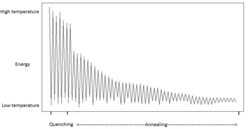
[image:5.612.86.476.243.439.2]In this work we aim to find a minimum feature subset for identifying four GBS subtypes from a 156-feature real dataset. This represents a combinatorial problem and to find a good approximation of the best solution the QSA metaheuristic was selected. QSA, shown in Algorithm 2, is a version of the SA algorithm which has two phases: Quenching and Annealing. Quenching phase is applied at a very high temperature which is rap idly reduced using an exponential function until a quasi-thermal equilibrium is reached. Quenching phase has shown to allow the exploration of a wider portion of the solution space than previous SA approaches did [32]. In Annealing phase the temperature is gradually reduced and therefore the exploration is performed at a slower pace, and so the solution space is scrutinized aiming to find the best solution. Figure 1 shows the temperature behavior in both Quenching and Annealing phases.
Figure 1. Temperature behaviour in Quenching and Annealing phases of QSA.
The classical SA algorithm receives as input a set X of m examples with n features. Classical SA requires a triplet composed of an Annealing schedule, an Energy function and a neighbour function. The Annealing schedule is defined by the initial temperature Ti, the final temperature Tf and the Annealing constant αAnnealing. These values control the pace and duration of the search. The Energy function evaluates the quality of a solution. The goal of SA is to optimize this function. In this particular problem we used the purity measure as the Energy Function. The neighbour function receives both the current solution and temperature as input and returns a new candidate solution that is nearby to the curre nt solution, in terms of the variation of features between both solutions. For high values of T a broader search in the dataset is performed to generate Si. For low values of T the search becomes almost local.
11-27. EDITADA. ISSN: 2007-1558.
Figure 2. Energy behaviour in Quenching and Annealing phases of the QSA.
QSA uses two extra parameters: a Quenching constan t α Quenching and τ. These parameters work together to reduce the temperature at a rapid pace until τ converges to ε. In addition, this particular implementation uses a cooling constant αVLT at very low temperatures, which enables the search space to be me ticulously traversed, which corresponds to performing a local search.
Algorithm 2: Quenching Simulated Annealing (QSA) Input:
Examples X = x1,…,xm
Ti, Tf, αQuenching, αAnnealing, αVLT, τ
begin 1) T = Ti
2) Sbest = random feature subset 3) WhileT > Tfdo
4) // Metropolis cycle 5) Repeat
6) Si = Neighbor(Sbest , T)
7) ΔE = Energy(Sbest , X) – Energy(Si , X) 8) If ΔE < 0 then
9) Sbest = Si
10) Else
11) If random(0,1] < then 12) Sbest = Si
13) End if 14) End if
15) Until thermal equilibrium is reached 16) If τ > ε then // Quenching phase 17) γ = 1 – T
18) T+1 = γ * αQuenching * T 19) τ = τ2
20) Else // Annealing phase 21) T+1 = αAnnealing * T 22) End if
23) IfT / Ti < 0.1 then // Very low temperatures phase 24) T+1=αVLT * T
11-27. EDITADA. ISSN: 2007-1558.
QSA, shown in Algorithm 2, begins initializing the value of T (line 1). A random feature subset is taken as an initial best solution Sbest (line 2). In this implementation the initial size of Sbest (between 2 and 156 variables inclusive) and their elements are randomly selected using the Mersenne-Twister pseudo random number generator. An external cycle is performed for controlling temperature variations until Tf (line 3) is reached. The Metropolis cycle (nested loop of lines 5-15) is performed until “thermal equilibrium" is reached. In this cycle, a neighbor solution Si is generated using Sbest and the value of T (line 6). The Neighbor function draws a new state Si based on the previous state Sbest where a number of features in Sbest is replaced with new features randomly taken from the original dataset depending on the current temperature T. For high values of T, a maximum of 80% of the features are replaced. For low values of T, a maximum of 20% of them are replaced. The difference in energy ΔE between Sbest and Si is calculated (line 7). If ΔE < 0, that is Si is a better solution than Sbest (line 8), then Si
becomes the best solution (line 9). If ΔE >= 0, it means Si is a worse solution than Sbest, then the best solution Sbest is replaced with Si only if a random number generated in the range [0,1) is less than
(lines 11-12). This step is fundamental in SA since it allows to escape from local minima by accepting worse solutions than the current one. When the Metropolis cycle is finished, the temperature new T is updated (lines 16-22). If τ > ε the Quenching phase is performed; on this phase T will be rapidly reduced due to the use of αQuenching constant. After a few iterations of the external cycle (line 3), τ converges to ε (lines 19-21). Right after that, the Annealing phase is performed; on this phase T is reduced at a slower pace (line 17). As stated before, this particular implementation of QSA uses a αVLT constant to perform local searches at very low temperatures (for T / Ti < 0.1) (lines 23-25). When T reaches Tf, QSA algorithm returns the feature subset that optimizes the energy function (line 27).
2.2.5 Description of QSA-PAM method
[image:7.612.78.543.399.531.2]The method we introduced in this work is a combination of two methods: Quenching Simulated Annealing (QSA) and Partitions Around Medoids (PAM), named QSA-PAM method (Figure 3). This is a novel method in machine learning implemented to search a large search space for a feature subset that leads to a good solution for a clustering problem. In our work, QSA -PAM was used to solve the problem of identifying four GBS subtypes - AIDP, AMAN, AMSAN and Miller-Fisher - with the highest purity possible. The method is described below.
Figure 3. QSA-PAM method.
QSA-PAM receives a dataset with n features as input. In this particular implementation n = 156. The class attribute was excluded as required in a clustering problem. We used it as the ground truth to compute the purity of the clusters obtained w ith PAM. For all experiments, the number of clusters requested to PAM algorithm was k = 4, as there are four GBS subtypes present in the dataset.
11-27. EDITADA. ISSN: 2007-1558.
As a result of the method we obtained a list of feature subsets that build four clusters with the highest purity possible for each value of i, each corresponding to a GBS subtype. In other words, the list contains the best 2-feature subset, the best 3-feature subset, and so on up to the best 156-feature subset.
In this study we perform a number of runs of QSA -PAM. For each run, we set a different seed. These seeds were generated using Mersenne-Twister pseudo random number generator [33]. Using a different seed for each run of QSA-PAM allows for QSA part of the method to generate different combinations of feature subsets from the search space to choose from.
3
Results
3.1 Determination of QSA parameters
For tuning the proposed algorithm, we started determining the initial and final temperatures Ti and Tf respectively used by QSA part of our method. These temperatures are computed as follows [25]:
max
( (
max))
Z
Ti
In P
Z
(5)
min
( (
min))
Z
Tf
In P
Z
(6)
Where ΔZmax and ΔZmin are the maximal and the minimal deterioration respectively, both of the energy function. Deterioration refers to changes in the Energy function, that is, the changes in purity at a n extremely high temperature and extremely low temperatures for ΔZmax and ΔZmin respectively.
P(ΔZmax) and P(ΔZmin) are the probabilities of accepting a new solution with ΔZmax and ΔZmin respectively. The probability of accepting a new solution is close to 1 at extremely high temperatures and close to 0 at extremely low temperatures [25].
To determine ΔZmax and ΔZmin, 30 runs of QSA-PAM were performed using random samples from the 156-feature dataset. Different arbitrary temperature values, in the range [7.674419x10⁶, 1x10⁻⁵] were used. An average value of 0.1372 was obtained for ΔZmax and 0.0088 for ΔZmin. Using both equations in 5 and 6 led us to temperatures of 1.376999x10⁶ for Ti and 7x10⁻⁴ for
[image:8.612.161.452.553.638.2]Tf. We used these values as approximations to the final temperatures. To verify the quality of these values, three different combinations of Ti and Tf were used and compared in 30 runs of QSA -PAM: the values obtained with equations 5 and 6 (Ti = 1.376999x10⁶ and Tf = 7x10⁻⁴), an arbitrary higher temperature combination (Ti = 1.5x10⁶ and Tf = 1x10⁻³) and other arbitrary lower temperature combination (Ti = 1x10⁶ and Tf = 1x10⁻⁵). The purity values obtained across 30 runs were averaged for every temperature combination. Results are shown in Table 1.
Table 1. Average purity over 30 runs of QSA-PAM using three different temperature configurations.
Ti Tf Average best
solution (purity) after 30 runs of
QSA-PAM
1.5x10⁶ 1x10⁻³ 0.7509
1.376999x10⁶ 7x10⁻⁴ 0.7564
1x10⁶ 1x10⁻⁵ 0.7881
11-27. EDITADA. ISSN: 2007-1558.
Table 2. Final values for QSA parameters.
Parameter Value
Ti 1x10⁶
Tf 1x10⁻⁵ αQuenching
αAnnealing αVLT
τ
0.7 0.985
0.99 0.9
3.2 Experimentation
3.2.1 Finding clusters using the 156-feature dataset
[image:9.612.125.479.362.538.2]The aim of the initial experiments was to analyse the behaviour of clusters using the whole 156-feature dataset. In order to achieve our goal, QSA-PAM was run 30 times using the 156-feature dataset, each run with a different seed. In each run, a list of the best feature subset for i equals 2 to 156 was obtained. Then, the purity of clusters obtained using each of the feature subsets was calculated. Finally, the average purity of clusters over 30 runs for each value of i was computed. The results are shown in Figure 4. The chart shows an initial ascending behaviour, a peak is reached approximately at I equals 30 and then the chart begins to slowly descend. The average purity values ranged in [0.75, 0.80]. We want to highlight that two featur e subsets in the feature space over 30 runs reached a maximum purity of 0.8527. Also, by looking at Figure 4 we identified the need of determining a proper number of features to be used to create clusters of high purity.
Figure 4. Average purity for each maximu m number of variables requested to the method across 30 runs .
3.2.2 Analysis of the size of the feature subsets selected by QSA-PAM
11-27. EDITADA. ISSN: 2007-1558.
Figure 5. Median of the number of features selected by the method across 30 runs .
3.2.3 Analysis of frequencies of features selected by QSA-PAM
[image:10.612.93.511.464.676.2]We also investigated the total frequency of selection by QSA -PAM for each feature in the dataset along the 30 runs, as shown in Figure 6. A ranking for all the 156 features was created based on these frequencies. That is, the feature on top of this ranking is the most frequently selected features. The highest frequency possible for any feature over 30 runs was 4650, that is 155 x 30 (155 total features, 30 runs). The highest frequency obtained for a feature was 2612. Five features stood out of all the 156 features reaching a frequency greater than 2000. These features were 14, 142, 13, 15 and 138 as shown in the c hart. We considered to use for further experiments only features with a frequency over 1000. This number of features counted to fifty. Coincidentally, fifty was the threshold derived from the analysis described in section 3.2.2.
11-27. EDITADA. ISSN: 2007-1558.
3.2.4 Quality of clusters formed using feature subsets based on the ranking of frequencies
[image:11.612.93.507.205.412.2]Based on the ranking of features according to frequencies for all 156 features, we created new datasets using the bes t 2 features, the best 3 features, and so on, up to 156 features. For each of these datasets, a distance matrix was computed using Gower's similarity coefficient. Each matrix was used as input for PAM to build four clusters. Finally, the purity of clusters was computed. The results of this experiment are shown in Figure 7. The highest purity obtained with these clusters was 0.81. This showed that not necessarily a sequential grouping of features based on the ranking of features would lead us to the desired purity of 1. Two other facts observed is that a low purity of 0.7054 is reached with few features (<=15) which is similar to that obtained (0.6976) with a large number of features (>=125).
Figure 7. Purity of clusters built using variables as ranked on the frequencies .
3.2.5 Finding clusters using the 50 most frequently selected features
11-27. EDITADA. ISSN: 2007-1558.
Figure 8. Average purity reached with the best 50 features according to frequency .
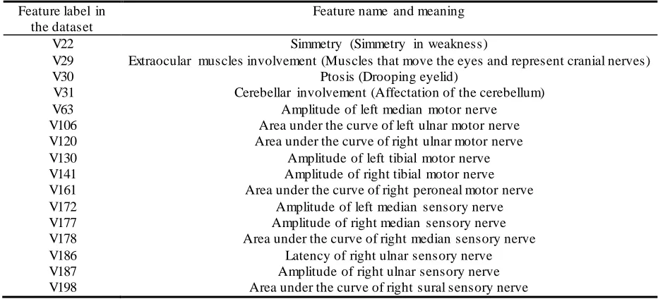
3.2.6 Our best 16-feature subset
In the second experiment of 30 runs, described in section 3.2.5, we found a feature subset that built four clusters with a purity of 0.8992. This subset contains 16 features: four clinical features and 12 features from the nerve conduction test . These features are listed in Table 3. We will further investigate this feature subset to create a predictive model.
Table 3. List of features that built 4 clusters with a purity of 0.8992.
Feature label in the dataset
Feature name and meaning
V22 Simmetry (Simmetry in weakness)
V29 Extraocular muscles involvement (Muscles that move the eyes and represent cranial nerves) V30
V31 V63 V106 V120 V130 V141 V161 V172 V177 V178 V186 V187 V198
Ptosis (Drooping eyelid)
Cerebellar involvement (Affectation of the cerebellum) Amplitude of left median motor nerve
Area under the curve of left ulnar motor nerve Area under the curve of right ulnar motor nerve
Amplitude of left tibial motor nerve Amplitude of right tibial motor nerve Area under the curve of right peroneal motor nerve
Amplitude of left median sensory nerve Amplitude of right median sensory nerve Area under the curve of right median sensory nerve
Latency of right ulnar sensory nerve Amplitude of right ulnar sensory nerve Area under the curve of right sural sensory nerve
3.2.7 Statistical analysis
[image:12.612.72.538.357.569.2]11-27. EDITADA. ISSN: 2007-1558.
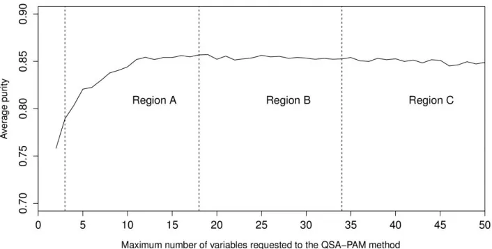
[image:13.612.125.478.129.308.2]According to the results shown in Table 4, we foun d statistical significant differences between purities achieved in regions B and C as shown in Figure 9. A more extensive search in these regions could lead to a better result. That is, requesting a number of variables to QSA-PAM between 19 and 34, or between 35 and 50.
[image:13.612.142.470.368.418.2]Figure 9. Regions of Average purity reached with the best 50 features
Table 4. Friedman-Holm test for regions A, B, and C.
Regions compared p Value Ho
A - B 0.317 Accepted
B - C 0.000 Rejected
A – C 1.000 Accepted
3.2.8 Temperature and energy behaviour in QSA
11-27. EDITADA. ISSN: 2007-1558.
Figure 10. Temperature behaviour in Quenching and Annealing phases of QSA-PAM for I = 50.
Figure 11. Energy behavior in Quenching and Annealing phases of QSA-PAM for i = 50.
4
Discussion
In this study we aimed to find a minimum feature subset to build four clusters, each corresponding to a GBS subtype, with the highest purity possible. In order to achieve our goal we introduced a combination of a metaheuristic (QSA) and a clustering algorithm (PAM), which we named QSA-PAM method.
[image:14.612.125.450.345.526.2]11-27. EDITADA. ISSN: 2007-1558.
The final feature subset identified in this study includes a combination of clinical and nerve conduction features. As to the four clinical features, they are reported in the literature as common clinical characteristics of GBS subtypes. This confirm the ability of QSA-PAM to select relevant clinical features for the identification of clusters. Concerning the electrophysiological features, further studies are required to confirm these findings. The identification of a minimum nerve conduction feature s ubset would be very useful to design a fast electrodiagnostic test.
On the other hand, this finding leads to the research question of the possibility of distinguishing the GBS subtypes investigated in this study with only one type of feature by itself, either clinical or nerve conduction feature. Specifically, a study to investigate the ability of clinical features to identify GBS subtypes is recommended. Wakerley et. al. [36] identified a set of clinical diagnostic features to classify GBS subtypes that could be used in the proposed research.
An important contribution of this study is a ranking of 156 features related with GBS. This ranking was created according to the frequency of selection of each feature by QSA -PAM across 30 runs. This ranking may be used in further studies.
With QSA-PAM, we found a 16-feature subset able to build four clusters present in our dataset with a purity of 0.8992. This finding, although able to be improved, shows the effectiveness of the method to find good solutio ns to clustering tasks involving feature selection.
5
Conclusions
We introduced a novel approach to find relevant features for building four clusters, each corresponding to a GBS subtype, with the highest purity possible. Our method consists of a combination of Quenching Simulated Annealing (QSA) and Partitions Around Medoids (PAM), named QSA -PAM method. Our study represents the first effort on applying computational methods to perform a cluster analysis to a real GBS dataset. An original 156-feature real dataset that contains clinical, serological and nerve conduction test data from GBS patients was used for experiments. Different feature subsets were randomly selected from the dataset using the QSA metaheuristic. New datasets created using the feature subs ets selected were used as input to PAM algorithm to build four clusters, corresponding to a specific GBS subtype each. Finally, purity of clusters was measured. An initial experiment consisting of 30 runs of QSA -PAM was performed. The frequency of selection of each feature across the 30 runs was computed. A new dataset was created using the resultant top fifty features from the initial experiment and used as input to a final experiment of 30 runs of QSA-PAM. Finally, a 16-feature subset was identified as the most relevant.
The method here proposed was able to find a 16-feature subset that could build four clusters, each corresponding to a GBS subtype, with a purity of 0.8992. This result verifies the ability of metaheuristics to find good solutions to co mbinatorial problems in large search spaces. In addition, given a statistical significance difference between two groups of purities was found, a more exhaustive search using the maximum number of variables requested to the method associated with those gro ups may lead to higher purity values.
In the short term, we will investigate the use of filters to reduce the original dataset prior to the use of QSA-PAM and analyse the results.
The results of this work may help GBS specialists to broaden the underst anding of the differences among subtypes of this disorder.
Authors’ Contribution and Acknowledgments
11-27. EDITADA. ISSN: 2007-1558.
References
1. Pascual Pascual, S. I.: Protocolos Diagnóstico Terapéuticos de la AEP: Neurología Pediátrica. Síndrome de Guillain -Barré, Asociación Española de Pediatría, Madrid, Spain (2008).
2. Kuwabara, S.: Guillain-Ba rré syndrome, Drugs, Vol. 64, No. 1 (2004) 597-610.
3. Uncini, A., Kuwabara, S.: Electrodiagnostic criteria for Guillain -Barré syndrome: A critical revision and the need for an update, Clinical neurophysiology, Vol. 123, No. 8, (2012) 1487-1495.
4. Zúñiga González, E.A., Rodríguez de la Cruz, A., Milán Padilla, J.: Subtipos electrofisiológicos del Síndrome de Guillain -Barré en adultos mexicanos , Revista Médica del IMSS, Vol. 45, No. 5 (2007) 463-468.
5. Yuki, N., Hartung, H.P.: Guillain-Barré Syndrome, The New England Journal of Medicine, Vol. 366, No. 24 (2012) 2294 - 2304.
6. Babkin, A. V., Kudryavtseva, T. J., Utkina, S. A.: Identification and Analysis of Industrial Cluster Structure, World Applied Sciences Journal, Vol. 28, No. 10 (2013) 1408-1413.
7. Webb, J. A., Bond, N. R., Wealands, S. R., Mac Nally, R., Quinn, G. P., Vesk, P. A., Grace, M. R.: Bayesian clustering with AutoClass explicitly recognizes uncertainties in landscape classification, Ecography, Vol. 30, No. 4 (2007) 526-536. 8. Arnaud, L., Haroche, J., Toledano, D., Cacoub, P., Mathian, A., Costedoat-Chalumeau, N., Le Thi Huong-Boutin,
D., Cluzel, P., Gorochov, G., Amoura, Z.: Cluster analysis of arterial involvement in Takayasu arteritis reveals symmetric extension of the lesions in paired arterial beds, Arthritis & Rheumatism, Vol. 63 (2011) 1136-1140.
9. Burgel, P.R., Paillasseur, J.L., Caillaud, D. , Tillie-Leblond, I. , Chanez, P. , Escamilla, R. , Court-Fortune, I., Perez, T. , Carré, P., Roche, N.: Clinical COPD phenotypes: a novel approach using principal component and cluster analyses, European Respiratory Journal, Vol. 36, No. 10 (2010) 531-539.
10. Williams-DeVane, C.R., Reif, D.M., Cohen Hubal, E., Bushel, P. R., Hudgens, E.E., Gallagher, J. E., Edwards, S. W.: Decision tree-based method for integrating gene expression, demographic, and clinical data to determine disease endotypes, BMC Systems Biology, Vol. 7 (2013).
11. Docampo, E., Collado, A., Escaramís, G., Carbonell, J., Rivera, J., Vidal, J., Alegre, J., Rabionet, R., Es tivill, X.: Cluster Analysis of Clinical Data Identifies Fibromyalgia Subgroups, PLoS ONE, 8 (2013).
12. Van Koningsveld, R., Steyerberg, E.W., Hughes, R.A., Swan, A.V., van Doorn, P.A., Jacobs, B.C..: A clinical prognostic scoring system for Guillain-Barré syndrome, The Lancet Neurology, 6 (7), 589 - 94 (2007).
13. Walgaard, C., Lingsma, H.F., Ruts, L., van Doorn, P.A., Steyerberg, E.W., Jacobs, B.C.: Early recognition of poor prognosis in Guillain-Barré syndrome, Neurology, Vol. 76, No. 11 (2011) 968 - 975 (2011).
14. Durand, M.C., Porcher, R., Orlikowski, D., Aboab, J., Devaux, C., Clair, B., Annane, D., Gaillard, J.L., Lofaso, F., Raphael, J.C., Sharshar, T.: Clinical and electrophysiological predictors of respiratory failure in Guillain -Barré syndrome: a prospective study, The Lancet Neurology, Vol. 5, No. 12 (2006) 1021-1028.
15. Paul, B.S., Bhatia, R., Prasad, K., Padma, M.V., Tripathi, M., Singh, M.B.: Clinical predictors of mechanical ventilation in Guillain-Barré syndrome, Neurology India, Vol. 60, No. 2 (2012).
16. Walgaard, C., Lingsma, H.F., Ruts, L., Drenthen, J., van Koningsveld, R., Garssen, M.J., van Doorn, P.A., Steyerberg, E.W., Jacobs, B.C.: Prediction of Respiratory Insufficiency in Guillain-Barré Syndrome, Annals of Neurology, 67 (6), 781 - 787 (2010).
17. Halkidi, M., Batistakis, Y., Michalis, M.: On Clustering Validation Techniques, Journal of Intelligent Information Systems, Vol. 17, No. 2-3 (2001) 107-145.
18. Wagstaff, K., Cardie, C., Rogers, S., Schroedl, S.: Constrained K-means Clustering with Background Knowledge, Proceedings of the Eighteenth International Conference on Machine Learning, 577 - 584 (2001).
19. Forestier, G., Gancarski, P., Wemmert, C.: Collaborative clustering with background knowledge, Data and Knowledge Engineering, Vol. 69, No. 2 (2010) 211-228.
20. Leng, M., Cheng, J., Wang, J., Zhang, Z., Zhou, H., Chen, X.: Active Semisupervised Clustering Algorithm with Label Propagation for Imbalanced and Multidensity Datasets, Mathematical Problems in Engineering, Vol. 2013 (2013) 1 - 10. 21. Zhu, M., Meng, F., Zhou, Y.: Semisupervised Clustering for Networks Based on Fast Affinity Propagation, Mathematical
Problems in Engineering, Vol. 2013, (2013) 1-10.
22. Kirkpatrick, S., Gelatt, C. D., Vecchi, M. P.: Optimization by simulated annealing, Science, 220, 671- 680 (1983).
23. Cerny, V.: Thermodynamical approach to the traveling salesman problem: An efficient simulation algorithm, Journal of Optimization Theory and Applications , Vol. 45 (1985) 41-51.
24. Metropolis, N., Rosenbluth, A.W., Rosenbluth, M. N., Teller, A. H., Teller, E.: Equation of State Calculations by Fast Computing Machines, The Journal of Chemical Physics , 21, 1087 -1092 (2004).
11-27. EDITADA. ISSN: 2007-1558.
26. Kaufman, L., Rousseeuw, P.: Clustering by means of medoids, in: Y. Dodge (Ed.), Statistical Data Analysis Based on the L1Norm and Related Methods, North-Holland, 405 -416 (1987).
27. Han, J., Kamber, M., Pei, J.: Data mining: concepts and techniques . Morgan Kaufmann, San Francisco (2012).
28. Manning, C.D., Raghavan, P., Schütze, H.: An introduction to information retrieval. Cambridge University Press, Cambridge (2009).
29. Boriah, S., Chandola, V., Kumar, V.: Similarity Measures for Categorical Data: A Comparative Evaluation. Proceedings of the SIAM International Conference on Data Mining, 243 - 254 (2008).
30. Gower, J.: A general coefficient of similarity and some of its properties, Biometrics, 27 (4), 857 - 871 (1971).
31. Chávez Esponda, D., Miranda Cabrera, I., Varela Nualles, M., Fernández, L.: Utilización del análisis de clusters con variables mixtas en la selección de genotipos de maíz. Revista Investigación Operacional, 30 (3), 209 - 216 (2010).
32. Frausto-Solis, J., Román, E.F., Romero, D., Soberon, X., Liñan -García, E.: Analytically Tuned Simulated Annealing Applied to the Protein Folding Problem. Proceedings of the 7th International Conference on Computational Science, Part II. ICCS '07 Springer-Verlag, Berlin, Heidelberg. 370 – 377 (2007).
33. Matsumoto, M., Nishimura, T.: Mersenne Twister: A 623-dimensionally Equidistributed Uniform Pseudo-random Number Generator. ACM Trans. Model. Comput. Simul., 8, 3 - 30 (1998).
34. Frausto-Solis, J., Sánchez-Pérez, M., Liñan-García, E., Sánchez-Hernández, J.P.: Threshold temperature tuning Simulated Annealing for Protein Folding Problem in small peptides . Computational and Applied Mathematics , 32, 471 - 482 (2013). 35. Frausto-Solis, J., SanVicente-Sánchez, H., Imperial-Valenzuela, F.: ANDYMARK: An Analytical Method to Establish
Dynamically the Length of the Markov Chain in Simulated Annealing for the Satisfiability Problem in Wang, T. D., et al. (Eds.) Simulated Evolution and Learning, vol. 4247 of Lecture Notes in Computer Science, Springer Berlin Heidelberg, 269 - 276 (2006).