1 2 3
ARE MOTORCYCLE COMMUTERS DIFFERENT TO THOSE WHO USE CAR OR
4
PUBLIC TRANSPORT?
5 6
7
Margaret O’Mahony, Corresponding Author
8
Centre for Transportation Research
9
Department of Civil, Structural & Environmental Engineering
10
Trinity College Dublin
11
Dublin 2
12
Ireland
13
Tel: +353 18962084, Email: [email protected]
14 15 16
Word count: 3,644 words text + 12 tables/figures x 250 words (each) = 6,644 words
17 18 19 20 21 22 23
Submission Date: 1st August 2016 24
1
ABSTRACT
2 3
Motorcycles, or powered two wheelers (PTW), have received less attention as a commuting
4
mode than others such as car, public transport and bicycle. More common in warmer countries
5
such as in southern European countries and in densely populated countries, their narrow size and
6
flexibility offer advantages to users in congested urban settings and in other environments too.
7
With recent evidence of increasing demand for more flexible modes e.g. shared bike schemes in
8
Europe, the research presented here looks at use of the motorcycle for work trips in a northern
9
European country - Ireland. One of the questions explored was to see if the profiles of
10
motorcycle work trip users were closer to that of other modes such as bicycle users or drive
11
alone car users - or if motorcycle users had a different profile entirely - as a means of better
12
understanding the potential of the motorcycle mode in satisfying particular user needs. The place
13
of work census data for 2011 was used to examine differences across a number of variables:
14
gender, age, household composition, industrial group, urban vs rural, number of students in
15
households and work trip travel time. The research also examines which of a number of variables
16
are most relevant in determining work trip mode choice with particular emphasis on
17
distinguishing the characteristics of motorcycle work trip users using a multinomial logistic
18
regression. The research finds that the motorcycle work trip user profile most closely resembles
19
drive alone car user profiles across a number of variables.
20 21 22
Keywords: motorcycle, flexible mode, work trips 23
INTRODUCTION
1
Urban traffic congestion continues to pose difficulties for transport users and for local
2
authorities. The marked recent growth in more flexible modes such as the bike-sharing
3
phenomenon demonstrate the latent demand for modes that are convenient, not only in space but
4
also in time. Modes that offer insulation against congestion continue to gain traction as
5
congestion continues to be an intractable aspect of most urban settings. Motorcycles or powered
6
two wheelers (PTW) are more flexible than the car mode particularly in countries where lane
7
splitting is allowed. In the case of Ireland, the Road Safety Authority (1) advises against lane
8
splitting citing significant dangers but strictly speaking it is not illegal and is commonly
9
practiced by motorcycle users. Motorcyclists are also allowed to use some bus lanes but
10
according to their local association many do not distinguish between those they are allowed to
11
use and those they are not and many tend to use all bus lanes (2).
12
Much of earlier research on motorcycles focused on their impact on air pollution but
13
more recent research looks at the impacts on congestion e.g. the work of the Department for
14
London in the UK which examined the journey time and emissions of PTWs in bus lanes (3). As
15
part of the work, police assigned riders to survey the routes with one PTW travelling in bus lanes
16
where available and a PTW and a car travelling in general traffic lanes. They found that PTW
17
using bus lanes, where available, took an average of 2 mins 29 secs per km compared with 2
18
mins 46 sec per km in general lanes – cars took on average 3 mins 55 sec per km on the same
19
route. In parallel, they found that PTW use of bus lanes cuts CO2 emissions by an average of 20
0.4% and 9% and NOx by an average of between 0.4% and 10.1%. (3). Other work in Belgium
21
examined the impact of modal shift on traffic flow and traffic congestion in a case study in which
22
the traffic on the Leuven-Brussels motorway journey was simulated and substitution of 10% of
23
cars by motorcycles. They found that there were 1,925 reduced vehicle hours in the modelled
24
scenario as a result. They also noted a 6% lower emission cost, 1% of which could be attributed
25
to the replacement of cars by motorcycles and 5% to the smoother traffic flow (4).
26
In 2002, Wigan (5) put forward the case for the use of motorcycles as an effective means
27
of transport with many valuable characteristics but a high level of vulnerability. At that stage, he
28
noted that the mode had yet to be taken seriously on an adequate scale, and the necessary
29
understanding of travel and choice characteristics was still wanting. In 2006, Bruge et al (6) 30
developed a motorcycle ownership model for the UK using data from the UK National Travel
31
Survey, the Family Expenditure Survey and a survey of motorcycle users. More recently again,
32
Rose et al (7) aimed to enhance understanding of the role of PTWs for commuting in the context
33
of large Australian cities using census data and a travel survey of motorcyclists. Despite issues
34
related to the difficulty in surveying motorcycle users, they found that survey respondents highly
35
valued the utilitarian benefits of PTW commuting such as free parking, travel time savings and
36
parking near their destination. They also found that that PTW users were predominantly male
37
and tended to be highly educated with high incomes.
38
Cirilli et al (8) examined spatial structure and CO2 emissions due to commuting in 39
analysis on Italian urban areas and noted a 6.96% of commuters using motorcycles there for
40
commuting; relatively high compared with other countries. Research in another southern
41
European country (9) in 2007, noted increased PTW ownership and related traffic. They noted
42
that there was a clear difference between vehicle ownership rates and vehicle usage rates per
43
vehicle type and found that mopeds and motorcycles are preferred for particular types of trips
44
e.g. travelling in residential areas and weekdays during daytime. PTW users avoided travelling
45
on motorways and at nighttime due to the perceived higher safety risks.
Ireland is an island on the west of Europe, with a population of 4.7 million. In 2011, 2.7
1
million people commuted to work, school and college with 66% of workers driving to work and
2
of those driving to work females exceeded males (10). Ireland is predominantly rural,
3
geographically speaking, but there are significant population centers in 5 cities. The Greater
4
Dublin area (a term used to describe the commuter belt around Dublin including neighboring
5
counties) currently has a population of 1.9 million and is described in European terms as a
6
medium-sized city.
7
When comparing the urban based travel characteristics with rural areas in Ireland, the
8
cities dominate in terms of public transport use with 21% of commuters in Dublin using it and
9
less than 6% in the other cities. Cycling to work was most popular in Dublin at 6% followed by
10
Galway at 5%. The commuter belt around Dublin is substantial and more than 1 in 7 within that
11
area had travel times of an hour or longer to their work place. At the other end of the spectrum,
12
in many rural based towns, between 40% and 50% of work trips were less than 15 mins (10).
13
The research presented here aims to supplement the work of previous researchers in
14
helping to better understand the profile of PTW users, in different locations and conditions. The
15
work uses data from the 2011 Irish census. The next section describes the methods used
16
followed by a presentation of the results. The paper ends with a summary of conclusions.
17 18
METHODS
19 20
Data
21
The data used in this study was taken from the 2011 census of the Irish population. The census is
22
conducted every five years by the Central Statistics Office (CSO) and includes all individuals
23
present in the country on that particular date. From the census data an anonymised set of records
24
called the Place of Work Census of Anonymised Records (POWCAR) database focuses on
25
transport related aspects of the country’s population (11). Personal, household and travel
26
characteristic variables are defined for each entry. These include age, gender, highest level of
27
education completed to date, socio-economic group, household composition, year household was
28
built, residential area type, mode of travel to work, school or college, time of departure to work,
29
school or college, journey time to work, school or college, number of cars or vans available for
30
use in the household, location of usual residence and location of place of work, school or college.
31
Respondents are responsible for reporting on the variables in the census. Unfortunately data on
32
income is not available.
33
Of the total 1,467,006 individuals making the work trip and included in the analyses,
34
7,619 individuals travel to work by motorcycle which is less than 1%. The frequency
35
distributions that follow below are presented in percentages rather than in absolute terms so that
36
observation of the overall profile per mode can be more easily interpreted and compared across
37
modes.
38 39
Statistical Analysis
40
Logistic regression can be used to predict a categorical dependent variable on the basis of
41
continuous and/or categorical independents, to determine the effect size of the independent
42
variables on the dependent and to rank the relative importance of the independent variables. It
43
applies maximum likelihood estimation after transforming the dependent into a logit variable.
44
The logit is a natural log of the odds of the dependent variable equalling the highest value and in
45
this way logistic regression estimates the odds of a certain event occurring. The predictive
46
success of the logistic regression can be assessed by looking at the classification table, showing
correct and incorrect classifications of the dependent variable. Goodness of fit tests used are the
1
likelihood ratio test and the Nagelkerke statistic (12). The logistic regression equation is:
2 3
𝑧 = 𝑏0+ 𝑏1𝑋1+ 𝑏2𝑋2+ ⋯ + 𝑏𝑘𝑋𝑘 (1)
4 5
where z = log odds of the dependent variable = ln(odds(event)) or the logit
6
b0 = constant 7
b1, b2, etc = logistic regression coefficients 8
X1, X2, etc = dependent variables. 9
Exp(b) is the odds ratio for an independent variable i.e. the natural log base e raised to
10
the power of b. The odds ratio is the factor by which the independent variable increases or (if
11
negative) decreases the log odds of the dependent variables. Exp(z) is the odds ratio of the
12
dependent variable, being the odds that the dependent variable equals the level of interest rather
13
than the reference level.
14
The likelihood is a probability that the observed values of the dependent may be
15
predicted from the observed values of the independents. The log likelihood (LL) is its log and
16
varies from 0 to minus infinity. LL is calculated in the modelling by iteration using maximum
17
likelihood estimation. Because -2LL has approximately a chi-square distribution, -2LL can be
18
used for assessing the significance of logistic regression. In general, as the model becomes
19
better, the -2LL will decrease in magnitude.
20 21
RESULTS AND DISCUSSION
22 23
Frequency Distribution Profiles
24
The frequency distribution profiles of user and household characteristics were first compared
25
across different modes to observe if motorcyclist work trip users and their households were
26
markedly different to those of other modes. The following variables were considered: number of
27
household residents, number of workers in households, number of students in households,
28
household composition, gender of work trip maker, highest education level, age, work trip
29
journey time and work trip departure time.
30
The frequency distribution of numbers in households against work trip mode is shown
31
in Figure 1 and they use the primary axis in the figure. The mean and confidence intervals (CI)
32
for analysis of variance (ANOVA) tests between the numbers of people in households for the
33
different work trip transport modes are also plotted on the figure using the secondary axis (F=
34
24613, P < 0.001). The frequency distribution profile is very similar for the motorcycle and drive
35
alone (single occupancy car use) groups and ANOVA post hoc tests confirm this with the CIs
36
overlapping as shown in the figure. The mean of the number of persons in households for the car
37
passenger group is much higher than for the other groups and that there are similarities between
38
the cycle and work from home groups with similar percentages of one person, two person etc
39
households in both.
40
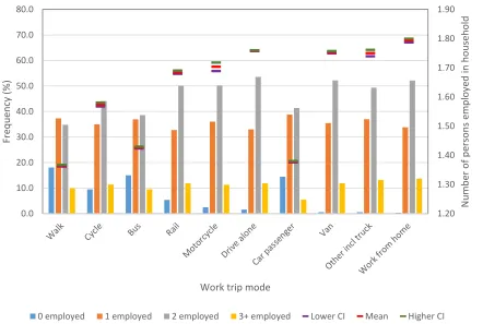
The second variable to be examined was the number of employed persons per
41
household. The frequency distribution and comparison of means by work trip transport mode is
42
presented in Figure 2. Some groups show more similarity with each other such as the rail and
43
motorcycle groups and separately the drive alone, van and other incl truck groups, as can be seen
44
in the overlap of CIs in Figure. (F = 15338, P < 0.001).
1
FIGURE 1 Frequency distribution and comparison of the means of number of persons in
2
households by work trip mode
3
4
FIGURE 2 Frequency distribution and comparison of mean numbers of persons employed
5
in households by work trip mode
6 7
2.50 2.70 2.90 3.10 3.30 3.50 3.70 3.90 4.10 4.30
0.0 10.0 20.0 30.0 40.0 50.0 60.0
N
u
m
b
er
o
f p
ers
o
n
s
in
h
o
u
se
h
o
ld
s
Fre
q
u
en
cy
(%
)
Work trip mode
1 person 2 person 3 person 4 person 5+ person Lower CI Mean Upper CI
1.20 1.30 1.40 1.50 1.60 1.70 1.80 1.90
0.0 10.0 20.0 30.0 40.0 50.0 60.0 70.0 80.0
N
u
m
b
er
o
f p
ers
o
n
s
em
p
loy
ed
in
h
o
u
se
h
o
ld
Fre
q
u
en
cy
(%
)
Work trip mode
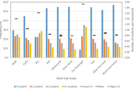
[image:6.612.85.527.374.671.2]The next variable under consideration was the number of students per household. The frequency
1
distribution is shown in Figure 3 and the CIs from the comparison of means analysis indicate that
2
the mean for the motorcycle group is statistically significantly similar to the drive alone, van and
3
work from home groups. (F = 51987, P < 0.001). The means of the number of students in
4
households in other groups such as the walk, cycle, bus and car passenger groups are found to be
5
higher and statistically significantly different to the motorcycle group.
6 7
[image:7.612.89.527.159.446.2]8 9
FIGURE 3 Frequency distribution and comparison of mean numbers of students in
10
households by work trip mode
11 12
Household composition was investigated next with the frequency distributions shown in Figure
13
4. Statistical comparison of means could not be conducted in this case due to the nature of the
14
categorisation. The drive alone, van, rail and motorcycle distributions are remarkably similar.
15 16
0.00 0.20 0.40 0.60 0.80 1.00 1.20 1.40 1.60 1.80 2.00
0.0 10.0 20.0 30.0 40.0 50.0 60.0
N
u
m
b
er
o
f stu
d
en
ts
p
er
h
o
u
se
h
o
ld
Fre
q
u
en
cy
(%
)
Work trip mode
1
FIGURE 4 Frequency distribution of household composition by work trip mode
2 3
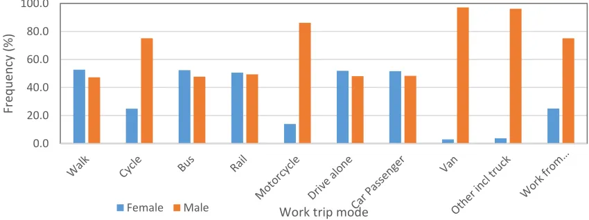
Six times the number of males compared with females use motorcycles to get to work, as can be
4
seen in Figure 5. Only the van and other incl truck groups show higher ratios of men to women.
5
A three-fold difference between males and females exists for the cycle and work from home
6
groups with a much more equal distribution between males and females evident for the walk,
7
bus, rail, drive alone and car passenger groups.
8 9 10
11 12
FIGURE 5 Frequency distribution of gender by work trip mode
13
0.0 10.0 20.0 30.0 40.0 50.0 60.0 70.0 80.0
Fre
q
u
en
cy
(%
)
Work trip mode Single Person
Lone parent with at least one resident child aged 19 or under
Lone parent with resident children but none aged 19 or under
Couple with at least one resident child aged 19 or under
Couple with resident children but none aged 19 or under
Couple with no resident children
Other Households
0.0 20.0 40.0 60.0 80.0 100.0
Fre
q
u
en
cy
(%
)
Work trip mode
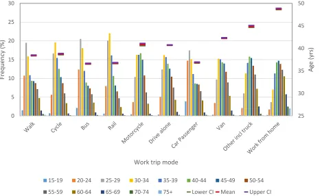
In Figure 6, the age frequency profiles for the motorcycle and drive along groups are similar and
1
the CIs of the means for the two groups overlap indicating a high degree of similarity. (F =
2
6064, P < 0.000). Higher proportions of walk, cycle, bus and rail groups are in the 20-35 age
3
groups with walk and cycle having somewhat higher age groups means than the bus and rail
4
groups. The working from home group has the highest mean age of 49 years.
5 6 7
[image:9.612.88.557.161.447.2]8 9
FIGURE 6 Frequency distribution and comparison of means for age by work trip mode
10 11
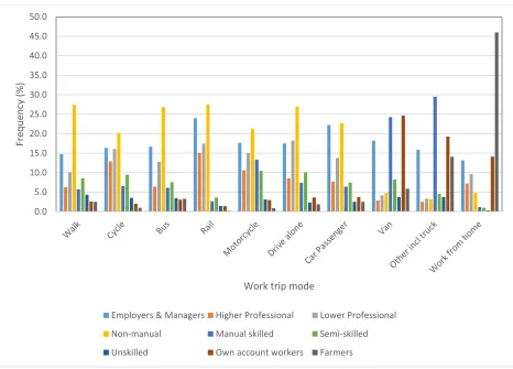
The frequency distributions for socio-economic group (SEG) by work trip mode are presented in
12
Figure 7. The distributions for the motorcycle, drive alone and car passenger groups have some
13
similarities but those for the other groups are more distinctive with less similarity appearing
14
between groups e.g. a relatively high proportion of higher professionals travel by rail with much
15
lower semi-skilled workers travelling by that mode.
16 17 18
25 30 35 40 45 50
0 5 10 15 20 25 30
Ag
e
(yrs
)
Fre
q
u
en
cy
(%
)
Work trip mode
15-19 20-24 25-29 30-34 35-39 40-44 45-49 50-54
1 2
FIGURE 7 Frequency distribution of socioeconomic groups (SEG) by work trip mode
3 4
Frequency distributions for work trip travel time are presented in Figure 8 along with the mean
5
and associated CIs for each mode. (F = 64320, P <0.000). Similar distribution shapes are evident
6
for the motorcycle, drive alone, van and other incl truck groups but markedly different profiles
7
exist for the walk, cycle and car passenger groups; all having very high proportions of trips
8
below 15 minutes. The rail group stands out with having the largest proportions of longer trips,
9
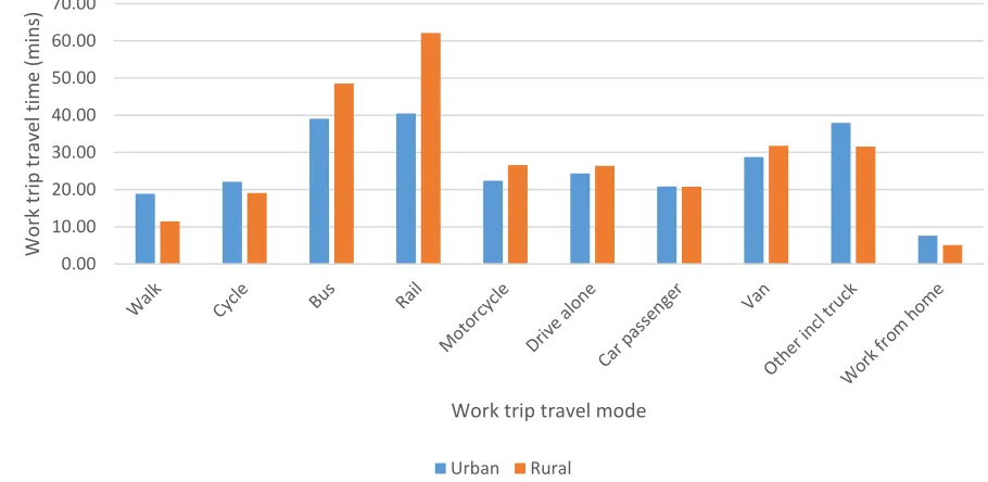
as might be expected. The difference in the means of work trip travel time between rural and
10
urban areas is shown in Figure 9. In most cases the urban trip is shorter than the rural trips. The
11
motorcycle and drive alone distances in both cases are closest when making a comparison across
12
the modes.
13 14
0.0 5.0 10.0 15.0 20.0 25.0 30.0 35.0 40.0 45.0 50.0
Fre
q
u
en
cy
(%
)
Work trip mode
Employers & Managers Higher Professional Lower Professional
Non-manual Manual skilled Semi-skilled
1
FIGURE 8 Frequency distribution and comparison of means for work trip travel time by
2
work trip mode
3 4
5 6
FIGURE 9 Means of work trip travel time for urban and rural based trips by work trip
7
mode
8 9 10
0.00 10.00 20.00 30.00 40.00 50.00 60.00
0.0 10.0 20.0 30.0 40.0 50.0 60.0 70.0 80.0 90.0 100.0
Wo
rk
t
rip
t
ra
ve
l t
im
e
(m
in
s)
Fre
q
u
en
cy
(%
)
Work trip mode
0-15 mins 16-30 mins 31-45 mins 46-60 mins 61-90 mins 91-180 mins Lower CI Mean Higher CI
0.00 10.00 20.00 30.00 40.00 50.00 60.00 70.00
Wo
rk
t
rip
t
ra
ve
l t
im
e
(m
in
s)
Work trip travel mode
[image:11.612.76.531.406.628.2]Multinomial Logistic Regression Results
1
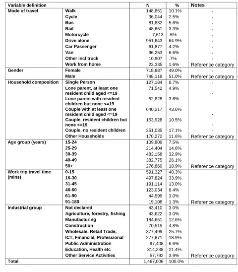
A multinomial logistic regression (MNL) analysis was set up with mode of travel as the
2
dependent variable and gender, household composition, age, work trip travel time and industrial
3
group as independent variables. Variable definition and frequencies are presented in Table 1.
[image:12.612.62.542.151.699.2]4 5
TABLE 1 Variable definition and frequencies
6 7
Variable definition N % Notes
Mode of travel Walk 148,851 10.1% -
Cycle 36,044 2.5% -
Bus 81,832 5.6% -
Rail 48,651 3.3% -
Motorcycle 7,613 .5% - Drive alone 951,643 64.9% - Car Passenger 61,877 4.2% -
Van 96,253 6.6% -
Other incl truck 10,907 .7% -
Work from home 23,335 1.6% Reference category
Gender Female 718,887 49.0% -
Male 748,119 51.0% Reference category Household composition Single Person 127,184 8.7% -
Lone parent, at least one resident child aged <=19
71,542 4.9%
- Lone parent with resident
children but none <=19
52,828 3.6%
- Couple with at least one
resident child aged <=19
640,217 43.6%
- Couple, resident children but
none <=19
153,928 10.5%
- Couple, no resident children 251,035 17.1% -
Other Households 170,272 11.6% Reference category Age group (years) 15-24 109,809 7.5%
25-29 214,404 14.6% 30-39 483,158 32.9% 40-49 382,775 26.1%
50+ 276,860 18.9% Reference category Work trip travel time
(mins)
0-15 591,327 40.3%
16-30 497,824 33.9% 31-45 191,114 13.0%
46-60 123,034 8.4%
61-90 44,599 3.0%
91-180 19,108 1.3% Reference category Industrial group Not declared 43,410 3.0%
Agriculture, forestry, fishing 43,622 3.0% Manufacturing 184,651 12.6% Construction 70,515 4.8% Wholesale, Retail Trade, 377,499 25.7% ICT, Financial, Professional 277,871 18.9% Public Administration 97,408 6.6% Education, Health etc 314,238 21.4%
Other Service Activities 57,792 3.9% Reference category
Total 1,467,006 100.0%
1
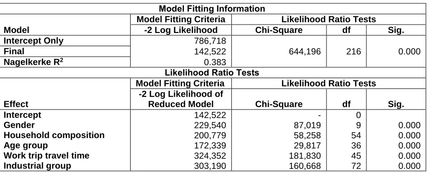
The model fitting information from the MNL regression are presented in Table 2. The
2
Nagelkerke R2 value of 0.383 represents relatively decent sized effects (12) and the table shows 3
that all of the variables included are significant. The reduction in the -2 log likelihood value for
4
the final model with the independent variables included compared with a model without them is
5
another indicator that the model improves with their addition. The larger the chi-square value,
6
the greater the loss of the model fit if that variable was dropped. In this case, dropping work trip
7
travel time would result in the greatest loss of model fit followed by industrial group, gender,
8
household composition and age group in that order.
9
Another useful measure to assess the utility of the model is classification accuracy
10
which compares the predicted group membership based on the logistic model with the actual.
11
The benchmark used here is that the model is considered useful if it shows a 25% improvement
12
over the rate of accuracy achievable by chance alone. The proportional by chance accuracy was
13
computed by calculating the proportion of cases for each group based on the number of cases in
14
each group for the dependent variable in Table 1 and then squaring and summing the proportion
15
of cases in each group; the result of which was calculated to be 0.44. The proportional by chance
16
accuracy criteria therefore = 1.25*0.44 = 54%. The classification accuracy rate from the model
17
was calculated to be 65.5% indicating that the model can be characterised as useful.
[image:13.612.74.507.345.521.2]18 19
TABLE 2 Model fitting information and statistical significance of independent variables
20 21
Model Fitting Information
Model
Model Fitting Criteria Likelihood Ratio Tests -2 Log Likelihood Chi-Square df Sig.
Intercept Only 786,718
Final 142,522 644,196 216 0.000
Nagelkerke R2 0.383
Likelihood Ratio Tests
Effect
Model Fitting Criteria Likelihood Ratio Tests -2 Log Likelihood of
Reduced Model Chi-Square df Sig.
Intercept 142,522 - 0
Gender 229,540 87,019 9 0.000
Household composition 200,779 58,258 54 0.000
Age group 172,339 29,817 36 0.000
Work trip travel time 324,352 181,830 45 0.000
Industrial group 303,190 160,668 72 0.000 22
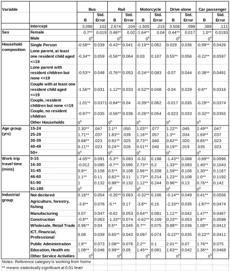
The results of the logistic regression model are presented in Table 3. The model examines the
23
factors that impact on mode choice and provides interesting insights into the impact of the
24
independent variables on mode choice for work trips. The value of -1.505 against females in the
25
first section indicates that they are less likely to use motorcycles to go to work than their
26
counterparts in the working from home category (reference situation). In the case of household
27
composition, motorcycle work trip users are least likely to be from households of couples with
28
young children 0.52) but interestingly bus users are even less likely to be from this group
(-29
1.56). As might be expected, individuals in younger age groups show a higher likelihood to use
30
motorcycles and the likelihood drops as age increases (1.03 and 1.16, respectively) but this
31
tendency is not exclusive to the motorcycle group. Not all of the B coefficients for work trip
32
travel time are statistically significant but of those that are motorcycle work trips are more likely
33
to be in the 16-30 min (2.73) and 31-45 min (2.66) journey time categories rather than in the
34
a strong relationship in this aspect. In terms of industrial group membership, motorcycle users
1
are least likely to work in the agricultural/forestry/fishing industries (-3.8) and most likely to
2
work in public administration or similar profession and education/health sectors.
[image:14.612.70.542.139.694.2]3 4
TABLE 3 MNL Parameter estimates
5 6
7 8
Variable
B
Std. Error B
Std. Error B
Std.
Error B
Std.
Error B
Std. Error
Intercept 3.096 .102 2.674 .104 -1.505 .215 3.506 .098 .389 .111
Sex Female 0.7** 0.019 0.48** 0.02 -1.64** 0.04 0.44** 0.017 1.0** 0.0193
Male 0b 0b 0b 0b 0b
Single Person -0.58** 0.039 -0.43** 0.041 -0.19** 0.062 0.029 0.036 -0.99** 0.0426
Lone parent, at least one resident child aged <=19
-0.34** 0.059 -0.56** 0.064 0.03 0.107 0.55** 0.056 -0.22** 0.0597
Lone parent with resident children but none <=19
-0.53** 0.048 -0.76** 0.053 -0.24** 0.083 -0.07 0.044 -0.38** 0.0491
Couple with at least one resident child aged <=19
-1.56** 0.031 -1.12** 0.033 -0.52** 0.048 -0.04 0.029 -0.6** 0.0316
Couple, resident
children but none <=19 -1.01** 0.037162500381579-0.84** 0.04 -0.39** 0.062 -0.017 0.035 -0.29** 0.0374 Couple, no resident
children -0.97** 0.035 -0.56** 0.036 -0.26** 0.054 -0.023 0.033 -0.32** 0.0355
Other Households 0b 0b 0b 0b 0b
15-24 2.30** .047 2.1** .050 1.03** .077 1.22** .045 2.49** .047
25-29 1.71** .037 1.83** .039 1.16** .057 1.3** .034 1.69** .037
30-39 0.68** .023 0.91** .025 0.73** .040 0.62** .020 0.65** .023
40-49 0.11** .023 0.24** .026 0.51** .040 0.19** .019 .035 .023
50+ 0b 0b 0b 0b 0b
0-15 -4.05** 0.091 -5.3** 0.093 -0.32 0.198 -1.43** 0.088 -0.89** 0.0996
16-30 -0.012 0.095 -0.7** 0.095 2.73** 0.2 1.33** 0.093 1.40** 0.1043
31-45 0.9** 0.108 0.5** 0.108 2.66** 0.208 1.59** 0.106 1.30** 0.1167
46-60 1.1** 0.11 0.82** 0.11 1.73** 0.214 1.23** 0.108 1.0** 0.1192
61-90 1 0.132 0.98** 0.132 1.12** 0.244 0.96** 0.13 0.76** 0.142
91-180 0b 0b 0b 0b 0b
Not declared 0.16** 0.054 -0.35** 0.063 -0.32** 0.106 -0.14** 0.049 0.41** 0.0556
Agriculture, forestry,
fishing -3.9** 0.076 -5.** 0.17 -3.8** 0.15 -2.33** 0.035 -1.87** 0.0474
Manufacturing 0.07 0.047 -0.02 0.053 0.64** 0.081 1.11** 0.042 1.47** 0.0467
Construction -0.9** 0.063 -1.33** 0.074 -0.62** 0.109 0.23** 0.053 0.8** 0.0598
Wholesale, Retail Trade 0.96** 0.04 0.5** 0.045 0.7** 0.075 0.88** 0.036 1.08** 0.0412
ICT, Financial,
Professional 0.08 0.039 0.65** 0.043 0.097 0.074 -0.22** 0.035 -0.22** 0.0411 Public Administration 1.8** 0.073 2.08** 0.076 2.2** 0.1 2.01** 0.07 1.76** 0.075
Education, Health etc 1.08** 0.046 0.99** 0.05 1.45** 0.081 1.63** 0.042 1.36** 0.0468
Other Service Activities 0b 0b 0b 0b 0b
Notes: Reference category is working from home ** means statistically significant at 0.01 level
Car passenger
Industrial group Household composition
Bus Rail Motorcycle Drive alone
Age group (yrs)
CONCLUSIONS
1
In the context of rising demand for more flexible modes, the paper seeks to understand the user
2
profiles of motorcycles for the work trip in the context of census data derived variables. The
3
results were made up of two parts 1) modal comparisons of variable frequency distributions and
4
2) results from a multinomial logistic regression analysis with mode of travel as dependent
5
variable and a number of socio-economic and work trip characteristics as independent variables.
6
The frequency distribution results show a high degree of similarity, and in most cases
7
statistically significant similarity, between the motorcycle group and single occupancy car trip
8
groups when comparing the following: number of persons in households, number of students in
9
household, household composition, age, socio-economic group and work trip travel time. In the
10
case of gender, the motorcycle group tends to be similar to the van and other including truck
11
group with a much higher number of males than females in those groups.
12
The multinomial logistic regression model found the independent variables made
13
statistically significant contributions to the model improving its classification accuracy
14
significantly over what would be achieved by chance. The chi-squared values indicated that
15
dropping work trip travel time would result in the greatest loss of model fit followed by
16
industrial group, gender, household composition and age group, in that order.
17
The model indicates motorcycle work trip users are least likely to be from households of
18
couples with young children and, as might be expected, individuals in younger age groups show
19
a higher likelihood to use motorcycles and the likelihood drops as age increases but this tendency
20
is not exclusive to the motorcycle group. Motorcycle work trips are more likely to be in the
16-21
30 min and 31-45 mins journey time categories rather than in the longer categories and these
22
large positive coefficients are the largest across the modes indicating a strong relationship in this
23
aspect. In terms of industrial group membership, motorcycle users are least likely to work in the
24
agricultural/forestry/fishing industries and most likely to work in public administration or similar
25
profession and in the education/health sectors.
1 2
REFERENCES
3 4
1. Road Safety Authority. Rules of the Road. www.rsa.ie. 2016. Accessed 20th July 2016. 5
2. MAG Ireland. The Irish Motorcyclists' Association. www.magireland.org. Accessed 20th
6
July 2016.
7
3. Transport for London. Motorcycle Policy Unit. Evaluation of Journey Time and Emissions
8
of PTWs in Bus Lanes, January 2011.
9
4. Yperman, I., Commuting by motorcycle: impact analysis, Transport & Mobility Leuven.
10
Belgium. 2011. Report 10, 69.
11
5. Wigan, M. Motorcycles as a Full Mode of Transportation, Transportation Research Record
12
1818, TRB, National Research Council, Washington, D.C., 2002, pp. 39-46.
13
6. Burge, P., Fox, J., Kouwenhoven, M., Rohr, C., Wigan, M. Modeling of motorcycle
14
ownership and commuter usage. Transportation Research Record, 2007, 2031, 59–68.
15
7. Rose, G. and Delbosc, A. Powered-two-wheelers for city commuting: Insight from
16
Australia's three largest capital cities. Journal of Transport Geography, 54. 2016., 325-335.
17
8. Cirrilli, A. and Veneri, P. Spatial Structure and CO2 emissions due to commuting: an 18
analysis on Italian urban areas. Quaderno di Ricerca n.253, 2010. Universita Politecnica
19
delle Marche.
20
9. Yannis, G., Golias, J., Spyropoulou, I., Papadimitriou, E., 2007. Mobility patterns of
21
motorcycle and moped riders in Greece. Transportation Research Record, 2007, 2031, 69–
22
75.
23
10. CSO (Central Statistics Office). Profile 10 Door to Door. 2012.
24
http://www.cso.ie/en/media/csoie/census/documents/census2011profile10/Profile_10_Full_ 25
Document.pdf
26
11. CSO Census 2011 Place of Work – Census of Anonymised Records (POWCAR). Central
27
Statistics Office, Ireland.
28
12. Field, A. Discovering statistics using IBM SPSS Statistics. 2012. 4th Edition. Sage 29
Publishing.