http://wrap.warwick.ac.uk
Original citation:
Rubio, Francisco J. and Steel, Mark F. J.. (2015) Bayesian modelling of skewness and
kurtosis with Two-Piece Scale and shape distributions. Electronic Journal of Statistics, 9
(2). pp. 1884-1912.
Permanent WRAP url:
http://wrap.warwick.ac.uk/75673
Copyright and reuse:
The Warwick Research Archive Portal (WRAP) makes this work of researchers of the
University of Warwick available open access under the following conditions.
This article is made available under the Creative Commons Attribution 2.0 Generic (CC
BY 2.0) license and may be reused according to the conditions of the license. For more
details see:
http://creativecommons.org/licenses/by/2.5/
A note on versions:
The version presented in WRAP is the published version, or, version of record, and may
be cited as it appears here.
Vol. 9 (2015) 1884–1912 ISSN: 1935-7524
DOI:10.1214/15-EJS1060
Bayesian modelling of skewness and
kurtosis with Two-Piece Scale and
shape distributions
F. J. Rubio and M. F. J. Steel
University of Warwick, Department of Statistics, Coventry, CV4 7AL, UK e-mail:francisco.rubio@warwick.ac.uk;M.F.Steel@stats.warwick.ac.uk
Abstract: We formalise and generalise the definition of the family of univariate double two–piece distributions, obtained by using a density– based transformation of unimodal symmetric continuous distributions with a shape parameter. The resulting distributions contain five interpretable parameters that control the mode, as well as the scale and shape in each direction. Four-parameter subfamilies of this class of distributions that cap-ture different types of asymmetry are discussed. We propose interpretable scale and location-invariant benchmark priors and derive conditions for the propriety of the corresponding posterior distribution. The prior structures used allow for meaningful comparisons through Bayes factors within flex-ible families of distributions. These distributions are applied to data from finance, internet traffic and medicine, comparing them with appropriate competitors.
AMS 2000 subject classifications:62E99, 62F15.
Keywords and phrases: Model comparison, posterior existence, prior elicitation, scale mixtures of normals, unimodal continuous distributions.
Received January 2015.
Contents
1 Introduction . . . 1885
2 Two-Piece Scale and shape transformations . . . 1886
2.1 Subfamilies with 4 parameters . . . 1888
2.2 Understanding the skewing mechanism induced by the proposed transformations . . . 1890
2.3 Reparameterisations . . . 1892
3 Bayesian inference . . . 1893
3.1 Improper priors and posterior propriety . . . 1893
3.2 Choice of the prior on (γ, δ, ζ) . . . 1895
3.3 Weakly informative proper priors . . . 1896
4 Applications . . . 1897
4.1 Internet traffic data . . . 1897
4.2 Actuarial application . . . 1898
4.3 Hierarchical Bayesian models in meta–analysis . . . 1901
4.3.1 Fluoride meta–analysis . . . 1901
5 Concluding remarks . . . 1903
Acknowledgements . . . 1904
Appendix . . . 1904
References . . . 1909
1. Introduction
We present a generalisation of the two-piece transformation defined on the fam-ily of unimodal, continuous and symmetric univariate distributions that contain a shape parameter. This generalisation consists of using different scale and shape parameters either side of the mode. We call this the “Double two-piece” (DTP) construction. The resulting distributions contain five interpretable parameters that control the mode and the scale and shape in each direction. This transfor-mation contains the original two-piece transfortransfor-mation as a subclass as well as a different class of transformations that only vary the shape of the distribution on each side of the mode. These two subclasses of distributions capture different types of asymmetry, recently denoted as “main-body skewness” and “tail skew-ness”, respectively, by Jones (2014b). Although some particular members of the proposed DTP family have already been studied (Zhu and Zinde-Walsh, 2009; Zhu and Galbraith,2010,2011), we formalise this idea and extend it to a wider family of distributions, analysing the types of asymmetry that these distribu-tions can capture. In addition, we propose and implement Bayesian methods for DTP distributions that allow us to meaningfully compare different distri-butions in these very flexible families through the use of Bayes factors. This directly sheds light on important features of the data. As a byproduct, we pro-pose a weakly informative prior elicitation strategy for the shape parameter of an arbitrary symmetric distribution. This strategy can be used, for example, to induce a proper prior for the degrees of freedom of the Student-t distribution.
et al. (1985); Haynes et al. (1997); Fischer and Klein (2004), and Klein and Fischer (2006). A third class of transformations consists of those that contain two parameters that are used for modelling skewness and kurtosis jointly. Some members of this class are the Johnson SU family (Johnson, 1949), Tukey-type
transformations such as theg-and-htransformation and the LambertW transfor-mation (Hoaglin et al.,1985; Goerg,2011), and the sinh-arcsinh transformation (Jones and Pewsey,2009). These sorts of transformations are typically, but not exclusively, applied to the normal distribution. Alternatively, distributions that can account for skewness and kurtosis can be obtained by introducing skewness into a symmetric distribution that already contains a shape parameter. Exam-ples of distributions obtained by this method are skew-t distributions (Hansen,
1994; Fern´andez and Steel, 1998a; Azzalini and Capitanio, 2003; Rosco et al.,
2011), and skew-Exponential power distributions (Azzalini,1986; Fern´andez et al.,1995). Other distributions containing shape and skewness parameters have been proposed in different contexts such as the generalized hyperbolic distribu-tion (Barndorff-Nielsen et al.,1982; Aas and Haff,2006), the skew–t proposed in Jones and Faddy (2003), and theα-stable family of distributions. With the exception of the so called “two–piece” transformation (Fern´andez and Steel,
1998a; Arellano-Valle et al.,2005), the aforementioned transformations produce distributions with different shapes and/or different tail behaviour in each direc-tion. Good surveys on families of flexible distributions can be found in Jones (2014b) and Ley (2015). Finally, alternative approaches used to produce flexible models are semi-parametric models (Quintana et al.,2009) or fully nonparamet-ric models (e.g.kernel density estimators and Bayesian nonparametric density estimation). Some advantages of the models studied in this paper are the in-terpretability of the parameters and the ease of implementation in different contexts.
In Section2, we present the DTP construction and discuss some of its proper-ties as well as two interesting subfamilies. We examine the nature of the asymme-try induced by these transformations and propose a useful reparameterisation. In Section 3 we present scale and location-invariant prior structures for the proposed models and derive conditions for the existence of the corresponding posterior distributions. Section 4contains three examples using real data. The first two examples concern the fitting of internet traffic and financial data, and we show how DTP distributions can be used to better understand the asym-metry of these data. In a second type of application we study the use of DTP distributions to model the random effects in a Bayesian hierarchical model. We compare various flexible distributions in this context, using medical data. Proofs are provided inAppendix.
2. Two-Piece Scale and shape transformations
Let F be the family of continuous, unimodal, symmetric densities ˜f(·;μ, σ, δ) with support onRand with mode and location parameterμ∈R, scale param-eterσ∈R+, and shape parameterδ∈Δ⊂R. A shape parameter is anything
Denote ˜f(x;μ, σ, δ) = 1
σf˜( x−μ
σ ; 0,1, δ)≡
1
σf( x−μ
σ ;δ). Distribution functions
are denoted by the corresponding uppercase letters. We define the two-piece probability density function constructed off(x;μ, σ1, δ1) truncated to (−∞, μ)
andf(x;μ, σ2, δ2) truncated to [μ,∞):
s(x;μ, σ1, σ2, δ1, δ2) =
2ε σ1
f
x−μ σ1
;δ1
I(x < μ)
+ 2(1−ε) σ2
f
x−μ σ2
;δ2
I(x≥μ), (1)
where we achieve a continuous density function if we choose
ε= σ1f(0;δ2) σ1f(0;δ2) +σ2f(0;δ1)
. (2)
We denote the family defined by (1) and (2) as the Double Two-Piece (DTP) family of distributions. The corresponding cumulative distribution function is then given by
S(x;μ, σ1, σ2, δ1, δ2) = 2εF
x−μ σ1
;δ1
I(x < μ)
+
ε+ (1−ε)
2F
x−μ σ2
;δ2
−1
I(x≥μ). (3)
The quantile function can be obtained by inverting (3). By construction, the density (1) is continuous, unimodal with mode atμ, and the amount of mass to the left of its mode is given byS(μ;μ, σ1, σ2, δ1, δ2) =ε. This transformation
preserves the ease of use of the original distribution f and allows s to have different shapes in each direction, dictated byδ1andδ2. In addition, by varying
the ratioσ1/σ2, we control the allocation of mass on either side of the mode.
The family F, on which the proposed transformation is defined, can be cho-sen to be, for example, the symmetric Johnson-SUdistribution (Johnson,1949),
the symmetric sinh-arcsinh distribution (Jones and Pewsey,2009), or the fam-ily of scale mixtures of normals, for which the density f with shape parameter δ can be written as f(xj;δ) =
∞
0 τ 1/2
j φ(τ
1/2
j xj)dPτj|δ for the observation xj,
where φ is the standard normal density and Pτj|δ is a mixing distribution on
R+. This is a broad class of distributions that includes,i.a.the Student-t
distri-bution, the symmetricα-stable distribution, the exponential power distribution (1 ≤ δ ≤ 2), the symmetric hyperbolic distribution (Barndorff-Nielsen et al.,
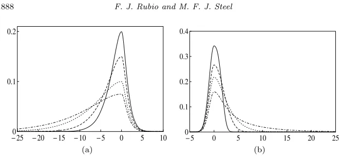
Fig 1. DTP sinh-arcsinh (DTP SAS) distribution withμ= 0and: (a)σ1= 2,3,5,7,σ2 =
1, δ1=δ2= 0.75; (b)σ1= 1,σ2= 2,δ1= 1,δ2= 1.5,1,0.75,0.5.
The DTP transformation preserves the existence of moments, if and only if they exist for bothδ1and δ2, since
Rx
rs(x;μ, σ
1, σ2, δ1, δ2)dx = 2ε
μ
−∞x
rf˜(x;μ, σ
1, δ1)dx
+ 2(1−ε)
∞
μ
xrf˜(x;μ, σ2, δ2)dx.
For example, iff in (1) is the Student-tdensity withδdegrees of freedom, then therth moment ofsexists if and only if bothδ1, δ2> r.
A random variable with density (1) can be decomposed as a variable that takes values distributed according to the density 2f(x;μ, σ1, δ1)I(x < μ) with
prob-ability ε, while taking values distributed according to 2f(x;μ, σ2, δ2)I(x≥μ)
with probability 1−ε. Other distributions allow for more tangible stochastic representations, but these representations are typically based on untestable as-sumptions. For example, the distribution of the underlying selection mechanism in hidden truncation models (Arnold and Beaver,2002), which include the skew-normal and skew-tdistributions of Azzalini (1985) and Azzalini and Capitanio (2003) cannot be tested in practice. In addition, not all kinds of asymmetry are generated by hidden truncation and, in most contexts, the interest is not in modelling the underlying selection mechanism. Jones (2014b) argues that, although it is useful to have a tangible generating mechanism, we are often only interested in modelling skewness and kurtosis properly, so that the flexibility and inferential properties of the final model might be more important than the availability of an intuitive generating mechanism.
2.1. Subfamilies with 4 parameters
Two-Piece Scale (TPSC) distributions
[image:6.612.164.497.91.243.2]s(x;μ, σ1, σ2, δ) =
2 σ1+σ2
f
x−μ σ1
;δ
I(x < μ)
+ f
x−μ σ2
;δ
I(x≥μ)
. (4)
The cases where f(·;δ) is a Student-t distribution or an exponential power distribution have already been analysed in some detail (Fern´andez et al.,1995; Fern´andez and Steel,1998a).
Two-Piece Shape (TPSH) distributions
An alternative subfamily can be obtained by fixingσ1=σ2=σin (1), implying
s(x;μ, σ, δ1, δ2) =
2ε σf
x−μ σ ;δ1
I(x < μ)
+ 2(1−ε)
σ f
x−μ σ ;δ2
I(x≥μ), (5)
where ε = f(0;δ2)
f(0;δ1)+f(0;δ2). This transformation produces distributions with
dif-ferent shape parameters in each direction. The variety of shapes obtained for different values of the parameters (δ1, δ2) depends, of course, on the choice of the
underlying symmetric modelf. Note also thatε, the mass cumulated to the left of the mode, differs from 1/2 wheneverf(0;δ1)=f(0;δ2). In the TPSH subclass
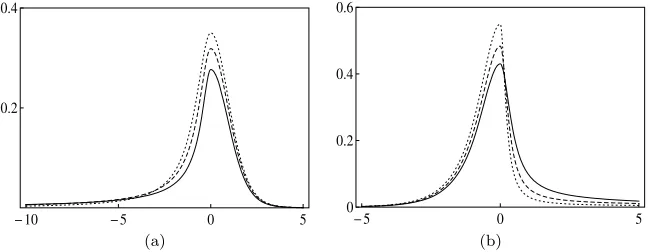
skewness can only be introduced if the shape parameters differ in each direc-tion. Other distributions with parameters that can control the tail behaviour in each direction have been proposed, for instance, in Jones and Faddy (2003); Aas and Haff (2006), and Jones and Pewsey (2009). Figure2shows two examples of distributions obtained with the TPSH transformation. Interchangingδ1and δ2
reflects the density function around the mode.
Fig 2. TPSH densities with(μ, σ) = (0,1): (a) TPSH Student-t,δ1= 0.25,0.5,1,δ2 = 10;
[image:7.612.117.442.501.627.2]2.2. Understanding the skewing mechanism induced by the proposed transformations
In order to provide more insight into the family of DTP distributions, we anal-yse the TPSC and TPSH families of distributions separately. For this purpose we employ two measures of asymmetry defined for continuous unimodal dis-tributions, the Critchley-Jones (CJ) functional asymmetry measure (Critchley and Jones, 2008) and the Arnold-Groeneveld (AG) scalar measure of skewness (Arnold and Groeneveld, 1995). These measures of asymmetry are based on quantiles of the distributions, so they do not require the existence of moments such as the Pearson measure of skewness or the standardised third moment. Here we focus on the use of AG and CJ as measures of asymmetry due to their interpretability and the fact they are always well-defined. The CJ func-tional measures discrepancies between points located on each side of the mode (xL(p), xR(p)) of the density g such that g(xL(p)) = g(xR(p)) = pg(mode),
p∈(0,1). It is defined as follows
CJ(p) = xR(p)−2×mode +xL(p) xR(p)−xL(p)
. (6)
Note that this measure takes values in (−1,1); negative values of CJ(p) indicate that the values xL(p) are further from the mode than the values xR(p). An
analogous interpretation applies to positive values. The AG measure of skewness is defined as 1−2G(mode), whereGis the distribution function associated with g. This measure also takes values in (−1,1); negative values of AG are associated with left skewness and positive values correspond to right skewness. For the DTP family in (1) these quantities are easy to calculate since AG = 1−2ε, and
CJ(p) =σ2f
−1
R (pf(0;δ2);δ2) +σ1f−
1
L (pf(0;δ1);δ1)
σ2fR−1(pf(0;δ2);δ2)−σ1fL−1(pf(0;δ1);δ1)
, (7)
where fL−1(·;δ) and fR−1(·;δ) represent the negative and positive inverse of f(·;δ), respectively. Note also that CJ(p) = AG whenδ1=δ2for everyp∈(0,1).
This means that for the TPSC family both measures coincide. In general, the AG measure of skewness can be seen as an average of the asymmetry function CJ (Critchley and Jones,2008). In the TPSC family, asymmetry is produced by varying the scale parameters on each side of the mode. This simply reallocates the mass of the distribution while preserving the tail behaviour and the shape in each direction. Since the nature of the asymmetry induced by the TPSC transformation is intuitively rather straightforward and has been discussed in
e.g.Fern´andez and Steel (1998a), we now focus on the study of TPSH transfor-mations.
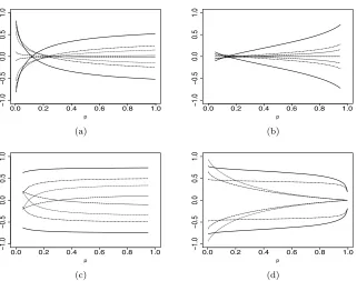
Fig 3. Asymmetry functional CJ for: (a) TPSH Student t; (b) TPSH exponential power;
(c) TPSH SMN-BS; (d) TPSH sinh-arcsinh distribution. Lines correspond toδ1 and δ2 as
in Table1and those values reversed.
Table 1
Parameters used to obtain the functionals in Figure3
TPSH Student-t TPSH sinh-arcsinh TPSH SMN-BS TPSH exp. power δ1 δ2 AG δ1 δ2 AG δ1 δ2 AG δ1 δ2 AG
1/10 10 −0.45 5 1 2/3 1 50 −0.44 1 2 0.11 1/2 10 −0.18 5 2 0.43 1 10 −0.09 1.5 2 0.03
1 10 −0.1 1 1/4 3/5 1 5 0.03 2 2 0
5 10 −0.01 1 1/2 1/3 2 1 −0.07 2.5 2 −0.01
varies from the tails to the mode of the density as a consequence of the different shapes and clearly the TPSH transformation is quite different from the TPSC one (for which CJ is constant). Figure3(c) corresponds to densities where CJ(p) changes sign for some combinations of the parameters (δ1, δ2) while retaining
[image:9.612.119.440.108.361.2]2.3. Reparameterisations
For the TPSC family (4), Arellano-Valle et al. (2005) propose the reparam-eterisation (μ, σ1, σ2, δ) ↔ (μ, σ, γ, δ) using the transformation σ1 = σb(γ),
σ2=σa(γ), where{a(·), b(·)} are positive differentiable functions, γ ∈Γ⊂R,
and the parameter space Γ depends on the choice of{a(·), b(·)}. The most com-mon choices fora(·) andb(·) correspond to theinverse scale factors parameter-isation {a(γ), b(γ)}={γ,1/γ}, γ∈R+ (Fern´andez and Steel, 1998a), and the
-skew parameterisation{a(γ), b(γ)}={1−γ,1 +γ}, γ∈(−1,1) (Mudholkar and Hutson, 2000). Jones and Anaya-Izquierdo (2010) and Rubio and Steel (2014) show that choosinga(γ) +b(γ) to be constant induces orthogonality be-tween σand γ. This reparameterisation is also appealing because the scalarγ can be interpreted as a skewness parameter since the CJ and AG measures of skewness depend only on this parameter. In particular, we obtain
AG = a(γ)−b(γ) a(γ) +b(γ).
Moreover, Klein and Fischer (2006) showed that the parameterγcan also be interpreted as a skewness parameter in terms of the partial ordering proposed by van Zwet (1964). This reparameterisation can also be used in DTP distri-butions for inducing orthogonality betweenσandγthrough parameterisations that satisfy a(γ) +b(γ) = constant. Under this reparameterisation, density (1) becomes
s(x;μ, σ, γ, δ1, δ2) =
2 σc(γ, δ1, δ2)
f(0;δ2)f
x−μ σb(γ);δ1
I(x < μ)
+ f(0;δ1)f
x−μ σa(γ);δ2
I(x≥μ)
, (8)
where c(γ, δ1, δ2) = b(γ)f(0;δ2) +a(γ)f(0;δ1). The interpretation of γ in the
wider DTP family is slightly different since the cumulation of mass (and thus AG) depends also on the shape parameters (δ1, δ2). However, the parameterγ
does not modify the shape ofs.
Using this reparameterisation we can obtain the “generalized asymmetric Student-t distribution” proposed in Zhu and Galbraith (2010) by takingf to be a Student-tdensity and{a(γ), b(γ)}={γ,1−γ},γ∈(0,1). Under the same parameterisation, the “generalized asymmetric exponential power distribution” proposed in Zhu and Zinde-Walsh (2009) corresponds to an exponential power density forf.
For the TPSH family (5) there seems to be no obvious reparameterisation that induces parameter orthogonality between the shape parameters and the other parameters. However, we can employ the reparameterisationδ1=δb∗(ζ),
δ2 = δa∗(ζ), with {a∗(·), b∗(·)} positive differentiable functions. This helps to
This reparameterisation can also be applied to the DTP family, leading to the following density
s(x;μ, σ, γ, δ, ζ) = 2 σc(γ, δ, ζ)
f(0;δa∗(ζ))f
x−μ σb(γ);δb
∗(ζ)I(x < μ)
+ f(0;δb∗(ζ))f
x−μ σa(γ);δa
∗(ζ)I(x≥μ)
, (9)
where c(γ, δ, ζ) =b(γ)f(0;δa∗(ζ)) +a(γ)f(0;δb∗(ζ)).
3. Bayesian inference
3.1. Improper priors and posterior propriety
In this section we propose a class of “benchmark” priors for the models studied in Section2with the parameterisations in (8) or (9). The proposed prior structure is inspired by the independence Jeffreys prior and the reference prior for the symmetric model, producing a scale and location-invariant prior.
The following result shows that the use of improper priors on the shape parameters of DTP models often leads to improper posteriors.
Theorem 1. Let x = (x1, . . . , xn) be an independent sample from (8) and consider the prior structure
p(μ, σ, γ, δ1, δ2)∝p(μ)p(σ)p(γ)p(δ1)p(δ2), (10)
where p(δ1)and/or p(δ2)are improper priors.
(i) Iff(0;δ)does not depend uponδ, then the posterior is improper.
(ii) If f(0;δ) is bounded from above, then a necessary condition for posterior propriety is
Δ
f(0;δi)np(δi)dδi<∞, i= 1,2. (11)
(iii) Iff(0;δ) is a continuous and monotonic function of δ, then for any 0≤ infδ∈Δf(0;δ)< M <supδ∈Δf(0;δ), a necessary condition for the
propri-ety of the posterior is
Δ
f(0;δi)n
[f(0;δi) +M]n
p(δi)dδi <∞, i= 1,2. (12)
Clearly, conditions (11) and (12) are satisfied whenp(δi) is proper fori= 1,2,
but they often do not hold under improper priors. Thus, Theorem 1 provides a warning against the use of improper priors on the shape parameters of DTP models. For instance, (i), (ii) and (iii) imply, respectively, that the use of im-proper priors on the shape parameters (δ1, δ2) of DTP exponential power (with
In the DTP model (8) the parameters γ and (δ1, δ2) control the difference
in the scale and the shapes either side of the mode, respectively. So we adopt a product prior structure p(γ)p(δ1, δ2), allowing for prior dependence between
δ1 and δ2. The following result provides conditions for the existence of the
corresponding posterior distribution whenf is a scale mixture of normals. The case where the sample contains repeated observations is covered as well. Theorem 2. Letx= (x1, . . . , xn)be an independent sample from (8). Letf be a scale mixture of normals and consider the prior structure
p(μ, σ, γ, δ1, δ2)∝
1
σp(γ)p(δ1, δ2), (13)
wherep(γ)andp(δ1, δ2)are proper.
(i) The posterior distribution of (μ, σ, γ, δ1, δ2)is proper if n≥2 and all the
observations are different.
(ii) If x contains repeated observations, let k be the largest number of obser-vations with the same value in x and 1 < k < n, then the posterior of
(μ, σ, γ, δ1, δ2)is proper if and only if the mixing distribution off satisfies
fori= 1,2 andj the observation index
0<τ1≤···≤τn<∞
τn−−(n−k 2)/2
j=n−k,n
τj1/2dP(τ1,...,τn|δi)dδi<∞. (14)
In the case of a two-piece Student-t sampling model,(14)is equivalent to
(k−1)/(n−k)+ξ
(k−1)/(n−k)
p(δi)
(n−k)δi−(k−1)
dδi <∞
and
(k−1)/(n−k)
0
p(δi)dδi= 0, (15)
for allξ >0 andi= 1,2.
For the reparameterisation (9), the parameters (γ, δ, ζ) have separate roles:γ controls the difference in the scale either side of the mode,δrepresents the shape parameter of the underlying symmetric density, andζcontrols the difference in the shape either side of the mode. For this reason, it is reasonable to adopt an independent prior structure on these parameters. The following result provides conditions for the existence of the posterior distribution.
Remark 1. Letx= (x1, . . . , xn) be an independent sample from (9). Let f be
a scale mixture of normals and consider the prior structure
p(μ, σ, γ, δ, ζ)∝ 1
σp(γ)p(δ)p(ζ), (16) wherep(γ),p(δ), andp(ζ) are proper. The posterior distribution of (μ, σ, γ, δ, ζ) is proper ifn≥2 and all the observations are different. If the sample contains repeated observations, we need to check that the induced prior on (δ1, δ2), for
the parameterisation (8), satisfies (14).
As discussed in previous sections, the parameters of a distribution obtained through the TPSC transformation, (μ, σ, γ, δ), can be interpreted as location, scale, skewness and shape, respectively. For this reason we adopt the product prior structure p(μ, σ, γ, δ) ∝ σ1p(γ)p(δ) for this family. In TPSH models the shape parameters (δ1, δ2) control the mass cumulated on each side of the mode
as well as the shape. In addition, these parameters are not orthogonal in general. We therefore adopt the product prior structurep(μ, σ, δ1, δ2)∝σ1p(δ1, δ2) in this
family, wherep(δ1, δ2) denotes a proper joint distribution which allows for prior
dependence betweenδ1 andδ2. Theorem2 covers the propriety of the posterior
under these priors for TPSC and TPSH sampling models. For TPSH models with the parameterisation (9), Remark1 provides conditions for the existence of the posterior distribution under the priorp(μ, σ, δ, ζ)∝σ1p(δ)p(ζ).
Another context of practical interest is when the sample consists of set ob-servations. A set observationSis simply defined as a set of positive probability under the sampling model, i.e.P[ObservingS] > 0. In particular, this corre-sponds to any observation recorded with finite precision, as well as left, right and interval censoring. When the quantitative effect of censoring is not negligi-ble, this must be formally taken into account. The following corollary provides conditions for the existence of the posterior from set observations with DTP sampling models.
Corollary 1. Letx= (S1, . . . , Sn)be an independent sample of set observations from (8). Let f be a scale mixture of normals and consider the prior structure
(13). Then, the posterior distribution of (μ, σ, γ, δ1, δ2) is proper if n≥ 2 and
there exists a pair of sets, say (Si, Sj), such that
inf
xi∈Si,xj∈Sj
|xi−xj|>0. (17)
Thus, whenever each sample of set observations contains at least two intervals that do not overlap, the posterior distribution of (μ, σ, γ, δ1, δ2) is proper. This
result also applies to the parameterisation (9) with prior (16).
3.2. Choice of the prior on (γ, δ, ζ)
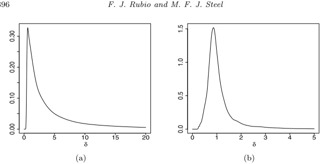
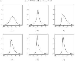
Fig 4. Priors forδ: (a) Student-tdistribution; (b) Sinh-arcsinh distribution.
bounded kurtosis measure, which is common to all models and is an injective function of δ, say κ = κ(δ). The boundedness assumption on κ allows us to assign a proper uniform prior on this quantity, while the injectivity is required for obtaining the induced prior on the parameterδ by inverting this function. See Critchley and Jones (2008) for a good survey on kurtosis measures.
We propose to adopt the scalar kurtosis measureκ= 2ff(mode)(πR) −1 from Critch-ley and Jones (2008), whereπR represents the positive mode of−f (the
inflec-tion point). This measure κ takes values in K ⊂ (−1,1), assigning the value κ = 0.213 to the normal distribution. Numerically, we have found that κ is an injective function of δ for many distributions f, such as the Student-t, the symmetric sinh-arcsinh, the symmetric Johnson-SU, the exponential power with
δ >1, the symmetric hyperbolic, the SMN-BS withδ <2.65, and the Meixner distribution. Another appealing feature of this measure of kurtosis is that both the AG skewness measure and κcan be interpreted as the average of certain functional measures of asymmetry and kurtosis using the same weight function (see Critchley and Jones,2008). Figure4shows the priors forδfor the Student-t and symmetric sinh-arcsinh distributions, induced by a uniform prior on the ap-propriate range forκ. The prior forδ in the Student-t model is an alternative to the Jeffreys prior in Fonseca et al. (2008) and is quite close to the gamma-gamma prior of Ju´arez and Steel (2010) with their parameterd= 1.2. It is also a continuous alternative to the discrete objective prior proposed in Villa and Walker (2014).
3.3. Weakly informative proper priors
[image:14.612.168.492.93.257.2]while for the scale parameter we employ a Half-Cauchy distribution with lo-cation 0 and scale s (Polson and Scott, 2012). Unfortunately, general choices for D and s are not available, given that these values depend on the units of measurement. We recommend conducting sensitivity analyses with respect to D and s. Note that the structure of this prior resembles that of the improper benchmark priors discussed in the previous sections.
This prior structure is also useful for choices of f that do not belong to the family of scale mixtures of normals and, consequently, the existence of the posterior under improper priors is not covered by the results in Subsection 3.1.
4. Applications
We present three examples with real data to illustrate the use of DTP, TPSC and TPSH distributions. We adopt the-skew parameterisation for DTP and TPSC models. In the first two examples, simulations of the posterior distributions are obtained using the t-walk algorithm (Christen and Fox, 2010). Given the hierarchical nature of the third example, we use the adaptive Metropolis within Gibbs sampler implemented in the R package ‘spBayes’ (Finley et al., 2007). R codes used here and the R-package ‘DTP’, which implements basic functions related to the proposed models, are available on request.
Model comparison within the DTP family is conducted via Bayes factors which are obtained using the Savage–Dickey ratio for nested models, and through importance sampling when we compare non-nested choices forf. We also com-pare the DTP model and its submodels with other distributions used in the literature. For a fair model comparison, we include appropriate competitors in each example, matched to the features of the data. A meaningful Bayesian com-parison with these other models would require the specification of priors for the parameters in these other distributions that are comparable (matched) to our models, and to compute Bayes factors we would need to use proper priors for all model-specific parameters. This would be a nontrivial undertaking and would risk diluting the main message of the paper. We choose instead to compare with these other classes of distributions through classical information criteria based on maximum likelihood estimates (MLE). We aim to show that the DTP fami-lies are flexible enough and then we can use formal Bayesian methods to select (or average) models within these families.
Given that DTP, TPSC, and TPSH distributions capture different sorts of asymmetry, conducting model comparison between these distributions not only provides information about which model fits the data better but it also indi-cates what kind of asymmetry is favoured by the data. In addition, the DTP family provides important advantages in terms of interpretability of parameters (and, thus, prior elicitation) and inferential properties.
4.1. Internet traffic data
Table 2
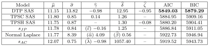
Internet traffic data: Maximum likelihood estimates, AIC and BIC (best values in bold)
Model μ σ γ δ ζ AIC BIC
DTP SAS 11.15 13.82 −0.98 12.95 −0.95 5849.03 5879.29 TPSC SAS 11.80 0.85 0.14 1.26 – 5884.95 5909.16 TPSH SAS 11.75 0.87 – 1.30 −0.08 5880.20 5904.41 sJ P 11.78 0.84 (ε)−0.16 1.25 – 5886.84 5911.05 Normal Laplace 11.77 8.39 (α) 4.09 (β) 0.56 – 5922.73 5946.94 sAC 12.07 0.75 (λ)−0.98 1057.40 – 5919.52 5943.73
bytes/sec within consecutive seconds. Ramirez-Cobo et al. (2010) propose the use of a Normal Laplace distribution to model these data after a logarithmic transformation. The Normal Laplace distribution is obtained as the convolution of a Normal distribution and a two–piece Laplace distribution with location 0 and two parameters (α, β) that jointly control the scale and the skewness. The Normal Laplace distribution has tails heavier than those of the normal distri-bution (Reed and Jorgensen,2004). We also use the sinh-arcsinh distribution of Jones and Pewsey (2009), indicated bysJ P and the skew-tof Azzalini and
Capi-tanio (2003), denoted bysAC(seeAppendix). Here, we explore the performance
of the DTP sinh–arcsinh distribution (DTP SAS). This distribution allows for all moments to exist and accommodates both heavier and lighter tails than the normal distribution, which is a submodel of the DTP SAS (δ1=δ2= 1,γ= 0).
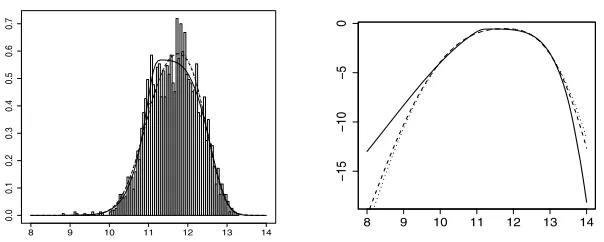
We use the priors of Subsection 3.3:μ∼Unif(0,25), σ ∼HalfCauchy(0, s), γ ∼ Unif(−1,1), ζ ∼Unif(−1,1), where s= 1/5,1,5 and for δ we adopt the prior in Figure4. The results were not sensitive to the choice ofs. Table2shows the MLE and the classical model comparison criteria for all models considered. The DTP SAS results indicate that the right tail is much lighter than that of the normal distribution, a feature that cannot be captured by the Normal Laplace distribution used in Ramirez-Cobo et al. (2010). In addition, there is strong evidence of “main-body” skewness, captured by different scales. Both features of the models are clearly important for these data and the DTP SAS model is strongly favoured by AIC and BIC. Bayes factors within the DTP SAS family also strongly support the most complete model, versus the possible submodels (all of them are < 10−100). Posterior predictive densities shown in Figure 5
illustrate how the DTP SAS model differs from the others in mode and tail behaviour (see the right panel).
4.2. Actuarial application
Fig 5. Internet traffic data (in logarithms; histogram) with (a) Predictive densities and
(b) Log-predictive densities: DTP (continuous line); TPSH (dashed line); TPSC (dotted line).
often used for budgetary planning, which emphasises the importance of properly modelling the tails of the distribution.
We explore two choices for f in (1): a Student-t distribution and an SMN-BS distribution (seeAppendix). We adopt the product prior structure (16) with uniform priors onγandζ. In order to produce matched priors onδfor these two models, we follow the strategy in Subsection 3.2. The measure of kurtosis κ∈ (0.213,0.633) for the Student-t model and κ∈ (0.213,0.560) for the SMN-BS model. Uniform priors forκinduce compatible priors forδin both models. Given that the data set contains a maximum number ofk= 30 repeated observations, we need to restrict the priors for (δ, ζ): for the Student-t model we truncate δ >2 and restrict ζ∈(−0.99,0.99). This truncation guarantees that condition (15) is satisfied since it implies thatδ1, δ2>(k−1)/(n−k)≈0.02. For the
SMN-BS model, the κ measure is injective only on the intervalδ ∈ (0,2.65), which covers the range κ ∈ (0.213,0.560). In addition, for this model we can check that condition (14) is satisfied if we truncate the δi’s away from zero, e.g. by
imposing δ > 1×10⁻⁶ and taking ζ ∈ (−0.999,0.999). Thus, we restrict the
prior forδin the SMN-BS model to (1×10−6,2.65). The posterior distributions
are proper by Remark1.
We also use the skew-tdistributions in Azzalini and Capitanio (2003) (sAC)
and Jones and Faddy (2003), denoted bysJF (seeAppendix). Table3shows the
[image:17.612.128.430.111.232.2]Table 3
Aon data: Maximum likelihood estimates, AIC and BIC (best values in bold)
Model μˆ σˆ ˆγ δˆ ζˆ AIC BIC
DTPt 7.93 1.61 −0.57 13.33 0.26 7283.1 7310.7 TPSCt 7.90 1.62 −0.59 10.98 – 7281.6 7303.6 TPSHt 9.13 1.46 – 9998.80 0.99 7434.4 7456.5 DTP SMN-BS 7.96 2.38 −0.48 0.46 −0.23 7280.6 7308.2 TPSC SMN-BS 7.90 2.36 −0.58 0.51 – 7279.4 7301.5 TPSH SMN-BS 8.03 3.43 – 0.31 −0.83 7280.1 7302.2
sJF 1.56 0.02 – (ˆa) 1560.6 (ˆb) 5.07 7302.1 7324.1
sAC 7.17 2.84 (ˆλ) 4.90 13.75 – 7280.7 7302.7
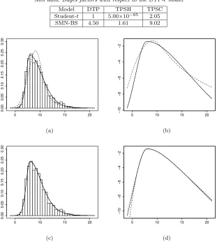
[image:18.612.177.488.258.605.2]Table 4
Aon data: Bayes factors with respect to the DTP-tmodel
Model DTP TPSH TPSC
Student-t 1 5.00×10−65 2.05
SMN-BS 4.50 1.61 9.02
Fig 6. Aon data (histogram) with (a) Predictive densities and (b) Log-predictive densities:
poor fit of the TPSHtmodel which clearly affects the estimation of the right-tail probabilities shown in Figure 6(b): this model produces a predictive probabil-ity of 0.01 for the event x > 17, while the other models lead to a predictive probability of less than 0.004. Unlike in the previous application, where right “main-body” skewness is combined with a heavier left tail (both γ and ζ are estimated to be highly negative), the skew-t by Azzalini and Capitanio (2003) does well here, as these data combine right skewness in the main body with a fatter right tail. This is a feature that the sAC imposes (for positiveλ with
both asymmetries in the opposite direction forλ <0). It is important to point out that the DTP families are not restricted in this way, as evidenced by the superiority of the DTP model in the previous application.
4.3. Hierarchical Bayesian models in meta–analysis
Bayesian hierarchical models are used in a variety of applied contexts to tackle parameter heterogeneity. A common example of this is the two–level normal model:
yj|θj ∼ N(θj, σj), j= 1. . . n,
θj ∼ N(μ, σ). (18)
A natural question is whether the assumption of normality of the random effects is appropriate: the implications of departures from this assumption are discussed in Zhang and Davidian (2001); Thompson and Lee (2008) and McCulloch and Neuhaus (2011).
In order to produce models that are robust to departures from normality of θj, several generalisations of (18) have been proposed. For example, Doss
and Hobert (2010) employ a Student–t distribution, Thompson and Lee (2008) use a TPSC tdistribution withδ >2 degrees of freedom, while Dunson (2010) follows a Bayesian nonparametric approach. The use of non–normal distribu-tional assumptions in this hierarchical model typically requires more sophisti-cated MCMC methods as discussed in Roberts and Rosenthal (2009).
4.3.1. Fluoride meta–analysis
In this example we analyse the data set presented in Marinho et al. (2003) and used in Thompson and Lee (2008), which contains n= 70 trials assessing the effectiveness of fluoride toothpaste compared to a placebo conducted between 1954 and 1994. The treatment effect is the “prevented fraction”, defined as the mean increment in the controls minus the mean increment in the treated group, divided by the mean increment in the controls. Thompson and Lee (2008) then propose the model
yj|θj ∼ N(θj, σj),
Fig 7. Predictive densities for the treatment effect: (a) Normal; (b) Symmetric SAS;
(c) TPSC normal; (d) TPSC SAS; (e) TPSH SAS; (f ) DTP SAS.
whereyj is the estimate of the treatment effect in studyj,θj is the true
treat-ment effect in studyj, and the parametersσj are estimated from the data and
assumed known. They compare the conclusions obtained for the true treatment effect for the following choices for P: (i) a TPSCt distribution withδ >2 de-grees of freedom, (ii) a symmetric Student tdistribution withδ >2 degrees of freedom, (iii) a TPSC normal distribution, and (iv) a normal distribution.
Here, we study six choices for P: (i) a normal distribution, (ii) a symmet-ric sinh–arcsinh (SAS) distribution, (iii) a TPSC normal distribution, (iv) a TPSC SAS distribution (Rubio et al., 2015), (v) a TPSH SAS distribution and (vi) a DTP SAS distribution. For the DTP model, we adopt the prior structure as in Subsection 3.3 p(μ, σ, γ, δ, ζ) =p(μ)p(σ)p(γ)p(δ)p(ζ) withμ ∼ Unif(−10,10), σ∼HalfCauchy(0, s), γ ∼Unif(−1,1), δ ∼p(δ), ζ ∼Unif(−1,1), with the prior shown in Figure 4 forδ, ands= 1/5,1,5. For the simpler sub-models we apply the same choices for the corresponding marginal priors. The results were not sensitive to the choice ofs.
[image:20.612.169.491.94.357.2]Table 5
Fluoride data: Bayes factors of submodels vs. the DTP SAS model
Model TPSH SAS TPSC SAS TPSC normal Sym. SAS normal
BF 1.27 0.30 0.05 0.02 5.2×10⁻⁵
However, the Bayes factors, shown in Table 5, slightly favour the TPSH SAS model, closely followed by the DTP SAS and the TPSC SAS models. Although the Bayes factors on the basis of this relatively small sample do not provide conclusive evidence about the best flexible model for the random effects, they definitely support asymmetric models with non-normal tails.
5. Concluding remarks
We discuss a simple, intuitive and general class of transformations (DTP) that produces flexible unimodal and continuous distributions with parameters that separately control main-body skewness and tails on each side of the mode. Al-though some particular cases of DTP models have already appeared (Zhu and Zinde-Walsh,2009; Zhu and Galbraith,2010), we formalise the idea and extend it to a wide range of symmetric “base” distributions F. We also distinguish two subclasses of transformations and examine their interpretation as skewing mechanisms. A considerable advantage of the DTP class of transformations is the interpretability of its parameters (see Jones, 2014b for the importance of interpretability) which, in the Bayesian context, also facilitates prior elicitation. We propose a scale and location-invariant prior structure and derive conditions for posterior existence, also taking into account repeated and set observations.
As illustrated by the applications, DTP families provide a flexible way of modelling unimodal data (or latent effects with unimodal distributions) and we provide a Bayesian framework for inference with sensible prior assumptions. In addition, we can conduct formal model comparison through Bayes factors for selecting models within the following classes:
• subclasses of DTP models with the same underlying symmetric base dis-tribution f: this is possible through the clearly separated roles of the parameters and the ensuing product prior structure with proper priors on γandζ.
• classes of DTP models with different underlyingf: in nested cases this is easy, given the separate roles of the parameters and the ensuing product prior structure with proper priors onδ, and in non-nested cases the priors on different shape parametersδare matched through a common prior on the kurtosis measureκ.
studied asymptotic properties of the maximum likelihood estimators (MLEs) for particular members of the DTP family (under the assumption of compactness of the parameter space). A more general study of the asymptotic properties of MLEs in DTP models represents an interesting research line.
DTP families can be extended to the multivariate case in several ways using general approaches. For TPSC models, Ferreira and Steel (2007) propose the use of affine transformations to produce a multivariate extension while Rubio and Steel (2013) propose to use copulas. In a similar fashion, the DTP (and consequently the TPSH) family can be used to construct multivariate distribu-tions.
A different subclass of DTP transformations can be obtained by fixingσ1=σ
andσ2= ff(0;(0;δδ21))σ, leading to distributions with different shapes but equal mass
cumulated on each side of the mode. This idea is proposed in Rubio (2013), who also composes this transformation with other skewing mechanisms to produce a different type of generalised skew-t distribution.
Rubio and Steel (2014) explore the use of Jeffreys priors in TPSC models. The use of Jeffreys priors for TPSH and DTP models is the object of further research.
Acknowledgements
We thank the Editor, an Associate Editor, and three referees for very help-ful comments. We gratehelp-fully acknowledge research support from EPSRC grant EP/K007521/1.
Appendix
Some density functions
Throughout we use the notationt= x−μσ .
(i) The symmetric Johnson-SU distribution (Johnson,1949):
˜
f(x;μ, σ, δ) = δ
σφ[δarcsinh (t)]
1 +t2−
1 2
.
(ii) The sinh-arcsinh distribution (Jones and Pewsey,2009):
sJ P(x;μ, σ, δ) =
δ
σφ[sinh (δarcsinh (t)−ε)]
cosh (δarcsinh (t)−ε) √
1 +t2 ,
where ε∈Rcontrols the asymmetry of the density and symmetry corre-sponds toε= 0.
(iii) SMN-BS, a scale mixture of normals with Birnbaum-Saunders(δ, δ) mixing:
˜
f(x;μ, σ, δ) = eδ12
√
δt2+ 1K 0
√ δt2+1
δ2
+K1
√ δt2+1
δ2
2πσδ3/2√δt2+ 1 .
(iv) The skew-tdensity from Jones and Faddy (2003):
sJF(x;μ, σ, a, b) =Ca,b−1
1 +√ t a+b+t2
a+1/2
1−√ t a+b+t2
b+1/2
,
wherea, b >0, andCa,b= 2a+b−1Beta(a, b)
√
a+b. The parameters (a, b) control the tails and skewness jointly. The densitysJF is asymmetric if and
only ifa=b, so that the density is skewed only when the tail behaviour differs in each direction.
(v) The skew-tdensity from Azzalini and Capitanio (2003):
sAC(x;μ, σ, λ, δ) = 2f(x;μ, σ, δ)F
λx
δ+ 1
δ+x2;μ, σ, δ+ 1
,
whereλ∈Randf andF are, respectively, the Student-tdensity function and the Student-t distribution function.
Proofs
In the proofs below, equation numbers other than (20) refer to equations in the main paper.
Proof of Theorem 1
The marginal likelihood of the data can be bounded from below as follows
m(x) ∝
Δ Δ Γ R+ R
⎡ ⎣n
j=1
s(xj;μ, σ, γ, δ1, δ2)
⎤
⎦p(μ)p(σ)p(γ)p(δ1)p(δ2)
dμdσdγdδ1dδ2
≥
Δ Δ Γ R+
x(1)
−∞
f(0;δ1)n
σnH(γ)n[f(0;δ
1) +f(0;δ2)]n
×
⎡ ⎣n
j=1
f
xj−μ
σa(γ);δ2
⎤
⎦p(μ)p(σ)p(γ)p(δ1)p(δ2)dμdσdγdδ1dδ2 (20)
where s(·) is given by (8) in the paper, H(γ) = max{a(γ), b(γ)}, and x(1)
represents the smallest order statistic of x. Therefore:
(i) follows by noting that the lower bound (20) does not depend uponδ1.
(ii) follows by using the following inequality, provided f(0;δ) ≤U for some U >0
f(0;δ1)n
[f(0;δ1) +f(0;δ2)]n
≥ f(0;δ1)n
2nUn ,
(iii) Given that f(0;δ) is continuous and monotonic, then for any 0 ≤ infδ∈Δf(0;δ)< M < supδ∈Δf(0;δ), there exists a set Δ2(M)⊂Δ such
that f(0;δ)< M for allδ∈Δ2(M). If we integrateδ2over Δ2, we obtain
the following lower bound, up to a proportionality constant, form(x)
Δ2 Δ Γ R+ x(1)
−∞
f(0;δ1)n
σnH(γ)n[f(0;δ
1) +f(0;δ2)]n
×
⎡ ⎣n
j=1
f
xj−μ
σa(γ);δ2
⎤
⎦p(μ)p(σ)p(γ)p(δ1)p(δ2)dμdσdγdδ1dδ2
≥
Δ2 Δ Γ R+ x(1)
−∞
f(0;δ1)n
σnH(γ)n[f(0;δ
1) +M]n
⎡ ⎣n
j=1
f
xj−μ
σa(γ);δ2
⎤ ⎦
× p(μ)p(σ)p(γ)p(δ1)p(δ2)dμdσdγdδ1dδ2.
From the last expression we obtain the necessary condition (12).
Analogous results can be obtained for δ2 by integrating μ over (x(n),∞),
wherex(n)represents the largest order statistic ofx.
Proof of Theorem 2
(i) In this parameterization,εin (2) does not depend onσ. This fact will be used implicitly in a change of variable below. We obtain
p(x)∝
Δ Δ
∞
0
∞
−∞ Rn
+
1 [a(γ) +b(γ)]n
n j=1λ
1 2 j
σn+1
× exp
⎡ ⎣− 1
2σ2
n
j=1
λj
ij(γ)2
(xj−μ)2 ⎤
⎦p(γδ1, δ2)
×
n
j=1
εdPλj|δ1I(xj < μ) + (1−ε)dPλj|δ2I(xj≥μ)
dμdσdγdδ1dδ2
≤
Δ Δ
∞
0
∞
−∞ Rn
+
1 [a(γ) +b(γ)]n
n j=1λ
1 2 j
σn+1
× exp
⎡
⎣− 1
2σ2h(γ)2
n
j=1
λj(xj−μ)2 ⎤
⎦p(γ)p(δ1, δ2)
×
n
j=1
εdPλj|δ1I(xj < μ) + (1−ε)dPλj|δ2I(xj≥μ)
dμdσdγdδ1dδ2,
whereij(γ) =a(γ)I(xj≥μ) +b(γ)I(xj< μ) andh(γ) = max{a(γ), b(γ)}.
upper bound can be written as follows
Δ Δ
∞
0
∞
−∞ Rn
+
h(γ)n
[a(γ) +b(γ)]n n
j=1λ
1 2 j
θn+1
× exp
⎡ ⎣− 1
2θ2
n
j=1
λj(xj−μ)2 ⎤
⎦p(γ)p(δ1, δ2)
×
n
j=1
εdPλj|δ1I(xj< μ) + (1−ε)dPλj|δ2I(xj≥μ)
dμdθdγdδ1dδ2.
By using that 0≤ε≤1, 12 ≤[a(γh)+(γb)(nγ)]n ≤1 it follows that the propriety
of the posterior of (μ, σ, γ, δ1, δ2) under this prior structure is equivalent to
the propriety of the posterior distribution of a TPSH sampling model with parameters (μ, σ, δ1, δ1) and prior structure π(μ, σ, δ1, δ1)∝σ−1p(δ1, δ2),
wherep(δ1, δ2) is a proper prior. The rest of the proof thus focuses on the
latter model, for which, by construction, we have
f(xj;μ, σ, δ1, δ2) =
∞
0
2λ12 j
√
2πσexp
− λj
2σ2(xj−μ) 2
× εdPλj|δ1I(xj < μ) + (1−ε)dPλj|δ2I(xj≥μ)
,
withεas in (2). Then, we can write the marginal ofx as follows
p(x) ∝
Δ Δ
∞
0
∞
−∞ Rn
+ n
j=1λ
1 2 j
σn+1
× exp
⎡ ⎣− 1
2σ2
n
j=1
λj(xj−μ)2 ⎤
⎦p(δ1, δ2)
×
n
j=1
εdPλj|δ1I(xj < μ) + (1−ε)dPλj|δ2I(xj ≥μ)
dμdσdδ1dδ2.
Separating the integral with respect to μ into n+ 1 integrals over the domains (−∞, x(1)), [x(1), x(2)), . . . , [x(n),∞), we have that
I1 =
Δ Δ
∞
0
x(1)
−∞ Rn
+ n
j=1λ
1 2 j
σn+1 exp
⎡ ⎣− 1
2σ2
n
j=1
λj(xj−μ)2 ⎤ ⎦
× p(δ1, δ2)(1−ε)n
n
j=1
dPλj|δ2dμdσdδ1dδ2.
I1 ≤ Δ
∞
0
∞
−∞ Rn
+ n
j=1λ
1 2 j
σn+1 exp
⎡ ⎣− 1
2σ2
n
j=1
λj(xj−μ)2 ⎤ ⎦
× p(δ2)
n
j=1
dPλj|δ2dμdσdδ2<∞.
The finiteness of this integral is obtained using Theorem 1 from Fern´andez and Steel (1998b). Now, using similar arguments we have that
I2 =
Δ Δ
∞
0
∞
x(n) Rn+ n
j=1λ
1 2 j
σn+1 exp
⎡ ⎣− 1
2σ2
n
j=1
λj(xj−μ)2 ⎤ ⎦
× p(δ1, δ2)εn
n
j=1
dPλj|δ1dμdσdδ1dδ2
≤
Δ
∞
0
∞
−∞ Rn
+ n
j=1λ
1 2 j
σn+1 exp
⎡ ⎣− 1
2σ2
n
j=1
λj(xj−μ)2 ⎤ ⎦
× p(δ1)
n
j=1
dPλj|δ1dμdσdδ1<∞.
Finally, for an intermediate region we have
I3 =
Δ Δ
∞
0
x(k+1)
x(k) Rn+ n
j=1λ
1 2 j
σn+1 exp
⎡ ⎣− 1
2σ2
n
j=1
λj(x(j)−μ)2
⎤ ⎦
× p(δ1, δ2)εk(1−ε)n−k
k
j=1
dPλj|δ1 n
j=k+1
dPλj|δ2dμdσdδ1dδ2
≤
Δ Δ
∞
0
∞
−∞ Rn
+ n
j=1λ
1 2 j
σn+1 exp
⎡ ⎣− 1
2σ2
n
j=1
λj(x(j)−μ)2
⎤ ⎦
× p(δ1, δ2)
k
j=1
dPλj|δ1 n
j=k+1
dPλj|δ2dμdσdδ1dδ2<∞.
The finiteness follows again from Theorem 1 from Fern´andez and Steel (1998b). Combining the finiteness ofI1,I2 andI3 the result follows.
(ii) This follows by using the previous proof together with Theorems 1, 2, and 3 from Fern´andez and Steel (1998b).
Proof of Corollary1
(μ, σ, δ), assuming thatS1, . . . , Sn is an i.i.d. sample of set observations from a
scale mixture of normalsf(·;μ, σ, δ) and adopting the priorπ(μ, σ, δ)∝σ−1p(δ),
where p(δ) is proper. The result then follows by combining this fact with The-orem 4 from Fern´andez and Steel (1998b).
References
Aas, K.and Haff, I. H. (2006), “The generalized hyperbolic skew student’s
t-distribution,”Journal of Financial Econometrics, 4, 275–309.
Arnold, B. C. and Beaver, R. J.(2002), “Skewed multivariate models
re-lated to hidden truncation and/or selective reporting (with discussion),”Test, 11, 7–54.MR1915776
Arnold, B. C. and Groeneveld, R. A. (1995), “Measuring skewness with
respect to the mode,”The American Statistician, 49, 34–38.MR1341197 Arellano-Valle, R. B., G´omez, H. W., and Quintana, F. A. (2005),
“Statistical inference for a general class of asymmetric distributions,”Journal of Statistical Planning and Inference, 128, 427–443.MR2102768
Azzalini, A.(1985), “A class of distributions which includes the normal ones,” Scandinavian Journal of Statistics, 12, 171–178.MR0808153
Azzalini, A.(1986), “further results on a class of distributions which includes
the normal ones,” Statistica, 46, 199–208.MR0877720
Azzalini, A.and Capitanio, A.(2003), “Distributions generated by
pertur-bation of symmetry with emphasis on a multivariate skew-t distribution,”
Journal of the Royal Statistical Society B, 65, 367–389.MR1983753
Barndorff-Nielsen, O., Kent, J., and Sørensen, M. (1982), “Normal
variance-mean mixtures andzdistributions,”International Statistical Review, 145–159. MR0678296
Berlaint, J., Goegebeur, Y., Segers, J., andTeugels, J.(2004), Statis-tics of Extremes: Theory and Applications, Wiley, New York.MR2108013 Christen, J. A. and Fox, C. (2010), “A general purpose sampling
algo-rithm for continuous distributions (thet-walk),” Bayesian Analysis, 5, 1–20.
MR2719653
Critchley, F.andJones, M. C.(2008), “Asymmetry and gradient
asymme-try functions: Density-based skewness and kurtosis,”Scandinavian Journal of Statistics, 35, 415–437.MR2446728
Doss, H. and Hobert, J. P. (2010), “Estimation of Bayes factors in a class
of hierarchical random effects models using geometrically ergodic MCMC al-gorithm,” Journal of Computational and Graphical Statistics, 19, 295–312.
MR2675092
Dunson, D. B. (2010), “Nonparametric Bayes applications to biostatistics,”
in: Bayesian Nonparametrics (Hjort, N. L., Holmes, C. C., M¨uller, P., and Walker, S. G., Eds.), pp. 223–273. Cambridge University Press, Cambridge.
MR2730665
Fern´andez, C., Osiewalski, J., andSteel, M. F. J.(1995), “Modeling and
Fern´andez, C.and Steel, M. F. J.(1998a), “On Bayesian modeling of fat
tails and skewness,”Journal of the American Statistical Association, 93, 359– 371.MR1614601
Fern´andez, C.and Steel, M. F. J.(1998b), “On the dangers of modelling
through continuous distributions: A Bayesian perspective”, in: Bayesian Statistics 6(Bernardo, J. M., Berger, J. O., Dawid, A. P., and Smith, A. F. M., Eds.), pp. 213–238. Oxford University Press (with discussion).
MR1723499
Fern´andez, C.andSteel, M. F. J.(2000), “Bayesian regression analysis with
scale mixtures of normals,”Econometric Theory, 16, 80–101.MR1749020 Ferreira, J. T. A. S.andSteel, M. F. J.(2006), “A constructive
represen-tation of univariate skewed distributions,”Journal of the American Statistical Association, 101, 823–829.MR2256188
Ferreira, J. T. A. S.andSteel, M. F. J. (2007), “A new class of skewed
multivariate distributions with applications to regression analysis,”Statistica Sinica, 17, 505–529.MR2408678
Finley, A. O., Banerjee, S., and Carlin, B. P. (2007), “spBayes:
An R package for univariate and multivariate hierarchical point-referenced spatial models,”Journal of Statistical Software, 19, 1–24.
Fischer, M. and Klein, I. (2004), “Kurtosis modelling by means of the
J-transformation,”Allgemeines Statistisches Archiv, 88, 35–50.MR2041425 Fonseca, T., Ferreira, M., and Migon, H. (2008), “Objective Bayesian
analysis for the student-t regression model,” Biometrika, 95, 325–333.
MR2521587
Goerg, G. M.(2011), “Lambert W random variables – a new generalized
fam-ily of skewed distributions with applications to risk estimation,”The Annals of Applied Statistics, 5, 2197–2230.MR2884937
Groeneveld, R. A.andMeeden, G.(1984), “Measuring skewness and
kur-tosis,”The Statistician, 33, 391–399.
Hansen, B. E.(1994), “Autoregressive conditional density estimation,” Inter-national Economic Review, 35, 705–730.
Haynes, M. A., MacGilllivray, H. L., and Mergersen, K. L. (1997),
“Robustness of ranking and selection rules using generalized g and k distributions,” Journal of Statistical Planning and Inference, 65, 45–66.
MR1619666
Hoaglin, D. C., Mosteller, F., andTukey, J. W.(1985),Exploring Data Table, Trends, and Shapes, Wiley, New York.
Johnson, N. L.(1949), “Systems of frequency curves generated by methods of
translation,”Biometrika, 36, 149–176.MR0033994
Jones, M. C. (2014a), “Generating distributions by transformation of scale,” Statistica Sinica, in press.
Jones, M. C. (2014b), “On families of distributions with shape parameters
(with discussion),”International Statistical Review, in press.
Jones, M. C., and Anaya-Izquierdo, K. (2010), “On parameter