University of Warwick institutional repository: http://go.warwick.ac.uk/wrap
A Thesis Submitted for the Degree of PhD at the University of Warwick
http://go.warwick.ac.uk/wrap/56806
This thesis is made available online and is protected by original copyright.
Please scroll down to view the document itself.
AUTHOR:Damon McDougall DEGREE: Ph.D.
TITLE:Assimilating Eulerian and Lagrangian Data to Quantify Flow Uncer-tainty in Testbed Oceanography Models
DATE OF DEPOSIT: . . . .
I agree that this thesis shall be available in accordance with the regulations governing the University of Warwick theses.
I agree that the summary of this thesis may be submitted for publication.
Iagreethat the thesis may be photocopied (single copies for study purposes only).
Theses with no restriction on photocopying will also be made available to the British Library for microfilming. The British Library may supply copies to individuals or libraries. subject to a statement from them that the copy is supplied for non-publishing purposes. All copies supplied by the British Library will carry the following statement:
“Attention is drawn to the fact that the copyright of this thesis rests with its author. This copy of the thesis has been supplied on the condition that anyone who consults it is understood to recognise that its copyright rests with its author and that no quotation from the thesis and no information derived from it may be published without the author’s written consent.”
AUTHOR’S SIGNATURE: . . . .
USER’S DECLARATION
1. I undertake not to quote or make use of any information from this thesis without making acknowledgement to the author.
2. I further undertake to allow no-one else to use this thesis while it is in my care.
DATE SIGNATURE ADDRESS
. . . .
. . . .
. . . .
. . . .
Assimilating Eulerian and Lagrangian Data to
Quantify Flow Uncertainty in Testbed
Oceanography Models
by
Damon McDougall
Thesis
Submitted to the University of Warwick
for the degree of
Doctor of Philosophy
Mathematics Institute
Contents
Acknowledgements iii
Declarations vi
Abstract vii
Notation viii
Chapter 1 Background and preliminaries 1
1.1 History of data assimilation . . . 1
1.1.1 Bayesian data assimilation . . . 2
1.1.2 Variational data assimilation . . . 5
1.2 Flavours of data assimilation . . . 6
1.2.1 Filtering and smoothing . . . 6
1.2.2 Eulerian and Lagrangian data assimilation . . . 8
1.3 Markov chain Monte Carlo methods . . . 9
1.3.1 Adaptive burn-in . . . 11
1.3.2 Metastability . . . 13
1.3.3 A note on random numbers . . . 15
1.4 Rigorous mathematical setting . . . 18
1.4.1 Regularity of random fields . . . 20
1.5 Thesis summary . . . 23
Chapter 2 Data assimilation for the advection equation 27 2.1 Overview . . . 27
2.2 Sampling the initial condition . . . 29
2.2.1 Varying step-size and observational error . . . 30
2.2.2 Varying the seed and sample size . . . 34
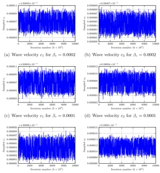
2.3 Sampling the wave velocity . . . 38
2.3.1 Simulated annealing . . . 44
2.4 Wavespeed mismatch . . . 46
2.4.1 Sampling the initial condition with model error . . . 50
2.5 Sampling the joint . . . 53
2.5.1 Seeding nearby the truth . . . 53
2.5.2 Slices of the objective function . . . 54
2.5.3 Seeding the wave velocity . . . 57
2.6 Modifying the likelihood . . . 58
2.6.1 Sampling the initial condition . . . 60
2.6.2 Sampling the wave velocity . . . 64
2.7 Conclusions . . . 68
Chapter 3 Data assimilation for controlled testbed ocean drifters 73 3.1 Overview . . . 73
3.2 Time-independent flow . . . 75
3.2.1 Na¨ıve control strategy . . . 76
3.2.2 A posteriori control strategy . . . 95
3.3 Periodic time-dependent disturbances . . . 99
3.3.1 Na¨ıve control for time-dependent flow model . . . 100
3.3.2 Time-dependent a posteriori control . . . 104
3.4 Conclusions . . . 111
Chapter 4 Data assimilation for optimally controlled testbed ocean drifters 114 4.1 Overview . . . 114
4.2 Derivation of control theory . . . 115
4.2.1 Optimal feedback control . . . 118
4.3 Specific use-case . . . 120
4.4 Application to data assimilation . . . 124
4.5 Conclusions . . . 126
Acknowledgements
First and foremost, I would like to thank both of my Ph.D supervisors, Professor
Chris Jones and Professor Andrew Stuart. They have not only provided invaluable
advice over the past four years, but have been an increasing source of encouragement,
support and understanding. Our feedback-oriented working relationship has pledged
staggeringly useful input, without which this doctoral work could not have been
completed. I feel tremendously privileged to have worked with two exceptionally
well-established scientists.
I have been fortunate to have had many inspirational scientific discussions with a
plethora of di↵erent people. These people all deserve thanks and they are, Tom Bellsky, Graham Cox, Sean Crowell, Masoumeh Dashti, Kody Law, Igor Mezi´c,
Lewis Mitchell, Richard Moore, Blane Rhoads, Naratip Santitissadeekorn, Elaine
Spiller and David White.
Practically, the computational resources managed by the University of Warwick’s
Centre for Scientific Computing have been paramount in the presentation of the
numerical material throughout this thesis. Thousands of hours of CPU time have
been utilised to complete this work and it does not go without profound gratitude.
Furthermore, I am very thankful for the funding provided by NERC and EPSRC to
undertake this research.
On a personal level, I must thank Sarah Chandler, Anna Clugston, Simon Cotter,
Martha Dellar, Andrew Duncan, Chris Cantwell, David Holmes, Dave Howden, Dave
years. Moreover, Andrew, Dave, Tom and Lewis deserve thanks, and probably a few
beers, for the daunting task of proofreading my work and taking immense pleasure
in telling me when I am wrong. Together with my girlfriend, Andrea Overbay, they
have provided an invaluable support network within which I sought solace where I
had problems, and delight where I succeeded.
Lastly, a debt of thanks is owed to my family. My parents, Tom and Eve, have
provided the requisite chromosomes needed to complete this work and, through
challenging me, my brother, Steven, has helped improve my skill of communicating
research level mathematics.
Mum and Dad, I have always appreciated your constant encouragement. The
emo-tional support you have given me will forever be appreciated. I feel privileged to
be your son and to share this great achievement with you. Though you have often
said, “I will never be able to understand what you do,” I am sure you will be proud
Declarations
Parts of the mathematical groundwork in Stuart [2010], which form the basis of
infinite dimensional Bayesian inverse problems, have been adapted for section 1.4.
The numerical studies and discussion done in sections 2.4 and 2.5.3, and related
conclusions in section 2.7, have been published jointly with Lee and Stuart in Lee
et al. [2011]. My primary contributions to the paper were on the numerical side,
and it is this aspect of the paper which I concentrate on in this thesis.
The e↵orts in chapter 3 are not yet published, but are a work in preparation with Jones in McDougall & Jones [2012].
The basis of chapter 4 concerns optimally controlled ocean gliders, the algorithm
for which was taken from Rhoads et al. [2010]. The underpinning theory for this
[Bryson Jr. & Ho, 1975] heavily inspired the mathematical presentation in section
4.2.
This work has not been submitted for a degree at any other university and, with
the exception of the four cases made above, I declare this research to be my own
Abstract
Data assimilation is the act of merging observed data into a mathematical model. This act enables scientists from a wide range of disciplines to make predictions. For example, predictions of ocean circulations are needed to provide hurricane disaster maps. Alternatively, using ocean current predictions to adequately manage oil spills has significant practical applications. Predictions are uncertain and this uncertainty is encoded into a posterior probability distribution. This thesis aims to explore two overarching aspects of data assimilation, both of which address the influence of the mathematical model on the posterior distribution.
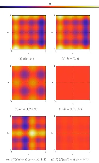
The first aspect we study is model error. Error is always present in mathematical models. Therefore, characterising posterior flow information as function of model error is paramount in understanding the practical implications of predictions. In a model describing advective transport, we make observations of the underlying flow at fixed locations. We characterise the mean of the posterior distribution as a function of the error in the advection velocity parameter. When the error is zero, the model is perfect and we reconstruct the true underlying flow. Partial recovery of the true underlying flow occurs when the error is rational, the denominator of which dictates the number of Fourier modes present in the reconstruction. An irrational error leads to retrieval only of the spatial mean of the flow.
Notation
S1: {x2R2 | kxk= 1} T2: R2/Z2
K2: Z2\ {(0,0)}
L2(T2): {f:T2 !R| RT2|f|2 <1} (also denotedL2per(T2))
H: {f 2L2(T2) | R
T2f = 0}
Hs orHpers : {f 2 H | Pk sk|hf, ki|2 <1}, where { k, k} are eigenvalues/eigenvectors
of the Laplacian that form a basis forH
⌘: Observational error
2: Variance of observational error
µ: Prior standard deviation
In: n⇥n identity matrix
↵: When used as an exponent, it refers to a regularity parameter. When used as a function,↵(·,·), it refers to an acceptance probability
µ0: The prior measure
µy: The posterior measure with observed data y
Chapter 1
Background and preliminaries
1.1
History of data assimilation
Consider a physical system describing some physical quantity of interest. Given noisy observations of the system’s state over time, the aim is to estimate the state of that system at some future time. This is a hard problem. For large weather systems, this problem has been looked at for decades and is still an active area of research. Estimating a future atmospheric or oceanic state is an endeavour that does not benefit solely scientists. The general public seek information in this regard and depend on the scientific community to produce predictions that are accurate, informative and actionable. Predictions regarding natural disasters are useful for national emergency services to mitigate potential fatalities. Predictions of weather in the short term aid in making safe and informed travel decisions. Predictions on a longer timespan, such as seasonal states for example, help companies execute profitable business manoeuvres. Predictions a↵ect people’s lives.
Data assimilation is the act of merging observations of some quantity into a mathe-matical representation of a physical system [Kalnay, 2002]. The result is an objective estimate of the state, which can be propagated through the model to obtain a pre-diction. There are many ways of utilising information from both observed data and model output, and this is reflected by the diverse history of data assimilation.
con-struct a ‘good’ initial condition to the model. Concon-structing such an initial condition will involve a mapping of the state inphysical space to a state inmodel space. One of the first to consider such mappings was Bergthorsson & Doos [1955] who explored interpolation of observational data onto a grid. Least-squares fitting [Gilchrist & Cressman, 1954; Cressman, 1959] also fits well within this objective. Methods on data analysis were used extensively before they inevitably merged with models to form what is termed today asdata assimilation. This is the act of taking observed data and a model to produce, in some sense, the ‘best possible’ prediction.
Rudolf Emil K´alm´an is probably the considered the forefather of state estimation. Most of the techniques all stem from one set of equations developed by Kalman in 1960, the Kalman Filter [Kalman, 1960]. One of the earliest physical applications of the Kalman filter was in trajectory estimation, leading to its implementation in the Apollo navigation computer; a key development in the Apollo program in the United States. It is worth noting that Swerling [Swerling, 1958] and Bucy [Kalman & Bucy, 1961] also contributed to a lot of the early theory.
1.1.1 Bayesian data assimilation
The Kalman filter can be derived explicitly from the following setup. We are given a linear process model on some statexk2Rn,
xk+1 =M xk, M 2Rn⇥n, k2N,
and noisy observations of the state,
yk=Hxk+⌘k, ⌘ki.i.d⇠ N(0, R),
at times k= 1, . . . , L. Here H is linear, called theobservation operator, and ⌘k is
theobservation error. The matrixR is the observation error covariance matrix. We then define two terms,mk|kandCk|k, the state estimate at timekgiven all the data
up to and including timek, and the error covariance of that state, respectively. The filter then proceeds in two steps, a prediction (or forecasting) step and an update (or analysis) step. The prediction step is as follows,
mk+1|k=M mk|k, (1.1a)
The variablesmk|k and Ck|k are often referred to as the analysis mean and analysis covariance. Furthermore, the variables mk+1|k and Ck+1|k are referred to as the
forecast mean and forecast covariance. The prediction formulae 1.1 indicate that the estimate of the state at time k+ 1 is simply the current state estimate propa-gated under the model M. Moreover, to obtain the covariance about the predicted state, one conjugates the current analysis covariance matrix by a forward model integration. These formulae are fairly intuitive. The interesting step is the update, where the analysis mean and covariance at timek+ 1 using a new observation have the following form,
mk+1|k+1 =mk+1|k+Ck+1|kH>(HCk+1|kH>+R) 1(yk+1 Hmk+1|k), (1.2a)
Ck+1|k+1 = (I Ck+1|kH>(HCk+1|kH>+R) 1
| {z }
Kalman gain matrix
H)Ck+1|k. (1.2b)
As we shall see later not only do (1.1) and (1.2) give a good state estimate for a linear system with Gaussian observation error, they are exactly the mean and covariance of Gaussian distributions about those states. They are called the prior distribution and posterior distribution respectively. The work of Kalman would form the basis of most data assimilation techniques for the next fifty years.
Data assimilation can be utilised in any model, though its most common applica-tion is to numerical weather predicapplica-tion (NWP). Several theoretical and numerical developments have taken place since the 1960s that have made data assimilation a more numerically tractable and stable process.
theoretically only applicable to linear and Gaussian models. Lots of variants have been devised to mitigate certain undesirable properties of the EnKF. For example, thelocalised ensemble Kalman filter [Anderson, 2003; Ott et al., 2004; Baek et al., 2006] addresses problems relating to the rank-deficiency of the ensemble covariance matrix. The square root formulation of the Kalman filter addresses computational speed and stability issues that arise when computing the covariance matrix [Carlson, 1973]. In 2001, theensemble transform Kalman filter (ETKF) was devised with the aim of speeding up the computation of the forecast covariance matrix; a desirable quality. It is even more useful when using this to assess the efficacy of locations of future observation stations, as described in Bishopet al. [2001]. Thelocal ensemble transform Kalman filter [Ott et al., 2004] allows massively parallel data assimila-tion schemes to take place by partiassimila-tioning the physical domain into smaller chunks, paving the way for even faster computation.
In all of these filters, some approximation is made. We either approximate the model by linearising it about the current analysis mean, or we approximate the analysis and forecast distribution by two moments; a mean and covariance. One last method we have not mentioned is theparticle filter. Methods like the particle filter and other particle method variants are not new methods designed for the purpose of solving the data assimilation problem, they are existing statistical techniques for sampling unknown probability distributions. Sampling probability distributions is a task physicists, chemists and biologists have been executing decades before statisticians started proving theoretical results regarding their behaviour. Section 1.3 explores this topic in more detail.
spaces, it is a well-known fact that particle filters perform extremely poorly [Bickel et al., 2008]. For an in-depth overview of the particle filter background material, see Doucetet al. [2001]. Recent advances in this field mean that problems in high dimensions can, to a certain degree, be mitigated [Leeuwen, 2010].
Note that all of the above methods are either ensemble based methods or methods derived directly from the original Kalman filter, both of which require the calculation of a, potentially, very large covariance matrix.
1.1.2 Variational data assimilation
Everything discussed hitherto has approached the problem from a Bayesian perspec-tive, involving the computation of aspects of some distribution of interest. There are other approaches to addressing the problem of assimilating observations into a model that is utilised more heavily within the circle of numerical weather prediction. Vari-ational methods; involving the (nonlinear) minimisation of some cost functional, is one such approach. It is worth noting here that Bayesian and variational approaches are very closely related. The cost functional is exactly the negative logarithm of the posterior probability density function.
A first variational approach to data assimilation, due to Hoke & Anthes [1976], em-ployed a nudging term to push predictions towards physical observations. Although crude, methods like this are not entirely uncommon and exist today [Leeuwen, 2010; Vanden-Eijnden & Weare, 2012] for use in highly nonlinear problems. Optimal in-terpolation was the next important scientific tool for numerical weather prediction and Lorenc [Lorenc, 1986] has been a figurehead in implementing the cornerstone data assimilation techniques such as optimal interpolation, 3D-Var and 4D-Var into the Met Office’s operational numerical weather prediction schemes.
The two main methods used today are 3D-Var (introduced into numerical weather prediction by Lorenc et al. [2000] and also used at NCAR in Boulder, Colorado [Barker, 2004]) and 4D-Var. The 3D-Var method minimises the cost functional over state vectorsx with a single observation vector y,
J(x) = 1
2kH(x) yk 2
R+
1 2kxk
2
B, (1.3)
Courtier, 1987] incorporates a sequential flavour and instead minimises the cost functional with observations that come in at certain times,
J(x) = 1 2
N
X
k=1
kHk(xk) ykk2R+
1 2kxk
2
B. (1.4)
Between observations, one executes a forecasting step.
There are several issues with both of these when the operators H and M are non-linear or when the observational noise is non-Gaussian. In these cases, one may use Gauss-Newton minimisation with the incremental 4D-Var proposed by Courtier et al. [1994] to achieve a reduction in computational cost by an order of magnitude over standard 4D-Var. Operationally, numerical weather prediction models are in-variably highly nonlinear, necessitating the use of approximate methods [Lawless et al., 2005a,b; Lawless & Nichols, 2006].
The last, and likely most important problem in data assimilation arises when the modelM does not generate the data ythat is being assimilated [Nichols & Griffith, 1996, 2000]. It is important to understand the role of getting the model wrong, as so frequently happens in the physical realm of numerical weather prediction. It is the job of mathematical modellers to construct such a model that is close to reality and computationally cheap to run. Examples of explorations of toy models can be found in Apte et al. [2008a], Cotter et al. [2009] Smith et al. [2009], Smith et al. [2011] and Leeet al. [2011].
1.2
Flavours of data assimilation
Many di↵erent types of data assimilation exist and it is important to illustrate their di↵erences. There are too many to list them all here, though we highlight the most influential, explaining the di↵erences in their methodology and goals. We also give real-world examples of their use when appropriate.
1.2.1 Filtering and smoothing
Say we are given a model and we are interested in the state of a system at time k. Say we are also given a vector of observations (y1>, . . . , yK>)>. The distribution of interest is, P⇣xk {yj}lj=0
⌘
. When l= k, this is called the analysis distribution, when l < k it is called the forecast distribution, and when l = K it is called the smoothing distribution. Filtering is the process of obtaining the analysis distribution iteratively.
1. Start withP⇣xk {yj}kj=0
⌘
2. Integrate model to obtainP⇣xk+1 {yj}kj=0
⌘
3. Assimilate to obtainP⇣xk+1 {yj}kj=0+1
⌘
4. Setk k+ 1. Go to 1.
Smoothing is the process of estimating the state using all possible data. Note, once an estimate to the state at timek,xk, has been obtained, all future state realisations
are determined by solving the model with initial condition xk. When the model is
deterministic, it is often the case that smoothers will estimate the initial condition x0, since the state path is thus entirely determined. Figure 1.1 illustrates, in a cartoon, the qualitative di↵erences between filtering and smoothing. We show here the mean of the forecast and analysis distributions. Notice that the filtering path is not ‘smooth’. The jumps in this path are when the analysis step takes place. The green dots indicate theanalysis mean.
analysis
forecast
(a) Filtering (b) Smoothing
Figure 1.1: Two data assimilation strategies: filtering and smoothing. The blue path is the prior state. The black crosses indicate the true state of the system.
The red dots are observations. In the case of filtering, the green path is the forecast and the green dots areanalyses. In the case of smoothing, the green path
is the analysis given all the observations.
analysis distribution at the final time t = K and the smoothing distribution on the final state are exactly the same, P⇣xK {yj}Kj=0
⌘
. An excellent overview of filtering and statistical techniques to solve these inverse problems can be found in Wikle & Berliner [2007]. This work sets up the Bayesian framework for data assimilation methods and gives derivations of the Kalman and related sequential data assimilation approaches, including particle filter methods. For the beginner, it is an informative introduction to the underpinning theory.
Filtering, by construction, is an ‘on-line’ process. Operationally, it necessitates a model integration to generate a forecast. When a new observation is made, com-putational linear algebra and minimisation techniques are executed to give the best estimate of the state given all of the observations up to and including the new one. Due to its sequential nature, filtering is the more commonly used data assimilation strategy, not only for its interest to scientists within numerical weather prediction centres, but also to the dynamical systems community. Dynamical systems are also prevalent in the next two comparisons on types of data; Eulerian observations and Lagrangian observations.
1.2.2 Eulerian and Lagrangian data assimilation
Eulerian observations are point observations of a field. These are utilised extensively in chapter 2 of this thesis and an example of their usage is given below. We noisily observe a velocity field,v, of a fluid atfixed points in space and time,
yjk =v(xj, tk) +⌘jk, ⌘jk i.i.d⇠ N(0, 2).
The observation stations in space are fixed and do not change in time. Lagrangian observations, on the other hand, are observation stations that move with the fluid,
yk=z(tk) +⌘k, ⌘ki.i.d⇠ N(0, 2I2),
wherez is the position of the observation station and satisfies,
˙
z=v(z, t). (1.5)
The most common use-case of these observations are in representing positions of passive tracers in a fluid.
Their di↵ering nomenclature seeks only to emphasise the distinction on the type of observations being assimilated. The same data assimilation techniques are applied with either type of observation by appending the model state with the equations for the motion of the particles (1.5) [Kuznetsov et al., 2003]. The di↵erence between the two setups is that even if the model governing the evolution of v is linear, the full coupled model of the flow and the tracers is often nonlinear. Assimilation of data into nonlinear models is an advanced topic that will be covered in chapter 3 of this thesis with application to a two dimensional kinematic travelling wave model.
The Lagrangian observation set-up fits in extremely well within the oceanographic objective of assimilating observations of buoys, drifters, tracers or gliders. Estimat-ing ocean flows and buoy trajectories has a long history, very similar to that of NWP and the general Kalman filter literature. First, a comparison of forecast errors in a barotropic open ocean model can be found in [Robinson & Haidvogel, 1981], with emphasis on how forecasts are sensitive to boundary information. Applications of the full Kalman filter with Lagrangian observations can be seen as early as 1982 [Barbieri & Schopf, 1982; Miller, 1986; Parrish & Cohn, 1985; Carter, 1989]. For a variational least-squares approach to eddy estimation, the reader is directed to [Robinson & Leslie, 1985]. A standard mathematical framework for assimilating Lagrangian observations appeared in 2003 [Kuznetsov et al., 2003]. Finally, Robel et al. [2011] exposes a novel approach to ocean current observations involving the treatment of sea turtles as Lagrangian observers.
1.3
Markov chain Monte Carlo methods
Markov chain Monte Carlo (MCMC) methods are a class of computational tech-niques for drawing samples from a unknown target distribution. Employing MCMC methods for the case where the target distribution is the posterior distribution, these methods can be used to do data assimilation. We give a general outline for MCMC methods in the finite dimensional case, we then generalise the approach to an in-finite dimensional setting. Inin-finite dimensional Monte Carlo schemes are employed heavily throughout this thesis.
distribution is hard to sample directly, and an approximate method must be utilised. The idea is to make draws from a distribution that is easier to probe, and apply a transformation to map the resulting samples to the target distribution. More specifically, we wish to construct a sequence {xk}k2N, called a Markov chain, such
that each xk looks like it was drawn from the target distribution, p(x). We dream
up a distribution that is easy to sample, called the proposal distribution, q(xk,·),
which may depend on the current state of the chain. The proposal distribution specifies the probability of transitioning to the next term in the sequence. Given the current state in the Markov chain isxk, we draw z⇠q(xk,·) and propose z as
the next state in the sequence. We then acceptzas the next state with probability,
↵(xk, z) = min
⇢
1,p(z)q(z, xk) p(x)q(xk, z)
. (1.6)
The next state in the Markov chain is then,
xk+1=
(
zwith probability ↵(xk, z)
xk with probability 1 ↵(xk, z).
The Markov chain with acceptance probability (1.6) is called the Metropolis-Hastings chain. This acceptance probability was chosen so that the resulting Markov chain satisfies a detailed balance property with respect to the unknown stationary mea-surep(x). Therefore, if it is the case that the Markov chain is alsoergodic, then the samples converge to the unique invariant distributionp(x).
Metropolis-Hastings samplers are characterised by their proposal distributions. Some of the most common choices are:
• Gibbs sampler (in two dimensions): Letx= (x1, x2). Choose a component (1 or 2) ofx and propose either z = (y, x2) or z= (x1, y), respectively, where y is sampled from eitherp(y|x2) or p(y|x1), respectively.
• Independence sampler: Labelled as such not because it produces independent samples fromp, but because the proposal distribution q(x, z) =q(z) is inde-pendent of the current state in the chain.
• Random walk sampler: Here the proposal distribution is chosen to be sym-metric,q(x, z) =q(z, x).
good computational performance, but due to the simplicity of the proposal density its theoretical properties are well understood. Random walk Metropolis-Hastings samplers have nice convergence properties and are, as a consequence, used exten-sively in practice. We shall use a random walk Metropolis-Hastings sampler for our purposes. If the current state in the Markov chain is xk, a typical random walk
proposal will look like,
w= (1 2)12xk+ ⇠, ⇠ ⇠N(0, C), (1.7)
where C is a specified covariance operator (see 1.4.1). The tuneable parameter is called the random walk step size, or the proposal step size. If = 0, the Markov chain does not propose a jump in the state space and instead proposes w = xk. Any reasonable acceptance probability calculation should almost surely
give an acceptance probability of 1 in this case. When = 1, the Markov chain takes no information of its current state and the acceptance probability should be some non-negative quantity less than or equal to 1.
Using this approach, one can draw samples from the posterior distribution, obtain-ing its shape exactly. This is of use when the posterior distribution is not a Gaussian and cannot be uniquely determined by its first and second moments. The applica-tion of MCMC methods to data assimilaapplica-tion is widespread. For examples of their use, see Cotteret al. [2012, 2009, 2010, 2011]; Stuart [2010]; Leeet al. [2011]; Apte et al. [2008b, 2007, 2008a]; Herbei et al. [2008]; Herbei & McKeague [2009]; McK-eagueet al. [2005]; Michalak [2003]; Kaipioet al. [2000]; Kaipio & Somersalo [2007]; Mosegaard & Tarantola [1995].
Metropolis-Hastings samplers have been researched extensively to assess and im-prove their performance greatly [Roberts, 1997; Roberts & Rosenthal, 1998, 2001; Beskoset al., 2009] since their development by Metropoliset al. [1953] and Hastings [1970]. In 2005, the scientific community saw the introduction of adaptive ap-proaches that drop the Markovian assumption but maintain the ergodicity property with improved convergence times [Atchad´e & Rosenthal, 2005; Atchad´e, 2006].
1.3.1 Adaptive burn-in
on the seed of the chain and can be very hard to determine objectively. As a consequence it is often chosen by trial and error. For example, if the seed lies in the tail of the posterior distribution, it will take a longer time for the chain to reach stationarity than when seeded at a mode. Figure 1.2 illustrates this e↵ect. Once
Figure 1.2: Initial transient behaviour of Markov chains
START
0
COMPUTE T ITERATIONS
COMPUTE AVERAGE ACC. PROB., ↵
max{0, inc} ↵<IS↵ 1?
IS
↵>↵2? min{1, + inc} YES
NO
[image:24.595.132.510.106.361.2]YES
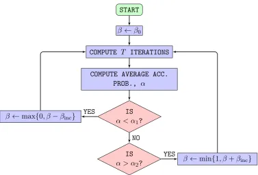
Figure 1.3: Flow chart detailing the adaptive scheme for
Observe that the initial step-size, 0, is too small and so the sampler takes sub-optimal jumps in the state space. The adaptive scheme adjusts the step-size to reach and maintain an acceptance probability of between 20% and 30%. After the burn-in, the adaptive scheme stops and the step-size is continued into the sampling part. Figure 1.4(b) shows that the acceptance probability maintains a steady value of about 25% after the burn-in.
1.3.2 Metastability
Looking at the form of the proposal for a random walk (1.7), it is clear that when
6
0 200 400 600 800 1000 Thousands of iterations (k⇥103)
0.0 0.2 0.4 0.6 0.8 1.0
↵(uk, z) 1 n
Pn
k=1↵(uk, z)
(a) Behaviour of the adaptive step-size scheme for inc= 10 4
0 200 400 600 800 1000
Thousands of iterations (k⇥103) 0.0
0.2 0.4 0.6 0.8 1.0
↵(uk, z) 1 n
Pn
k=1↵(uk, z)
(b) After burn-in the acceptance probability settles
Figure 1.5: Illustration of metastability in MCMC samplers
1.3.3 A note on random numbers
Monte Carlo methods require the use of randomly generated numbers. Any corre-lation within the generated variates can lead to an impeded convergence speed and severely bias computed moments.
Definition 1.3.1. Given some interval [a, b], let A=N\[a, b]. A pseudo-random number generator is a functionf :A!A. A seed for the random number generator is somex02A. Random numbers are produced by successively applyingf to obtain a sequencexn=f(xn 1), n= 1,2, . . ..
It is a property of all pseudo-random number generators that there exists N 2 N such thatxN =x0. In other words, pseudo-random number generators are periodic,
and the smallest such N is called the period. It is no surprise then, that random number generators will, by construction, never generate ‘truly’ random numbers. One can only hope their outputappears to be random. For this to hold,f should at least have a large period. For further sanity checks on randomness, a set of statistical tests have been devised to analyse various aspects of the output of pseudo-random number generators [Marsaglia, 1996].
by,
xn=s1n s2n s3n,
where,
s1n+1= (((s1n& 4294967294)⌧12) (((s1n⌧13) s1n) 19)),
s2n+1= (((s2n& 4294967288)⌧4) (((s2n⌧2) s2n) 25)),
s3n+1= (((s3n& 4294967280)⌧17) (((s3n⌧3) s3n) 11)).
The operators used above are defined as,
& : bit-wise AND : bit-wise XOR
⌧: bit-shift left (multiplication by 2)
: bit-shift right (division by 2, rounded down).
The Tausworthe generator presented here has a period of 288. This is noticeably smaller than that of the Mersenne-Twister algorithm, but it is a small price to pay given the greatly reduced computational cost involved in producing random variates with this method. The review in Jones [2010] is a notable work on the best practices of generating random numbers.
Random number generators like these produce uniformly distributed nonnegative integers between some constructed bounds. It is often the case that one wants random samples from the standard normal distribution. This can be achieved using a transformation that maps uniformly distributed variates to Gaussian distributed variates. The Box-Muller transform [Box & Muller, 1958] is such a transformation, and one of the most widely used ones.
Theorem 1.3.2(Box-Muller transform). LetU1andU2be two independent random variables drawn from the uniform distribution on [0,1]then
Z1=
p
2 log(U1) cos(2⇡U2), (1.8) Z2 =
p
2 log(U1) sin(2⇡U2), (1.9) are two independent random variables with standard normal distribution.
LetfZ1,Z2(z1, z2) be the joint probability density function of the pair (Z1, Z2). Writ-ingu1 = h11(z1, z2) and u2 =h21(z1, z2), we let fU1,U2(h11(z1, z2), h21(z1, z2)) be the joint probability density function of the pair (U1, U2). We use a standard change of variables relation,
fZ1,Z2(z1, z2) =fU1,U2(h11(z1, z2), h21(z1, z2))|det(J)|, (1.10) where, J = 0 B B @ @u1 @z1 @u1 @z2 @u2 @z1 @u2 @z2 1 C C A.
We invert (1.8)–(1.9) to obtainu1,
z12+z22 = 2 log(u1) cos2(2⇡u2) 2 log(u1) sin2(2⇡u2) = 2 log(u1),
) u1 = exp
✓
1 2(z
2 1 +z22)
◆
.
Similarly, to obtainU2,
z2 z1
= tan(2⇡u2)
) u2 = 1
2⇡arctan z2 z1 .
The Jacobian has determinant,
|det(J)|= det z1exp 1
2(z12+z22) z2exp 12(z12+z22)
z2
2⇡(z2 1+z22)
z1
2⇡(z2 1+z22)
!
= z
2 1 2⇡(z2
1 +z22) exp
✓
1 2(z
2 1+z22)
◆
+ z
2 2 2⇡(z2
1 +z22) exp
✓
1 2(z
2 1+z22)
◆
= 1 2⇡exp
✓
1 2(z
2 1 +z22)
◆
Finally, substituting into (1.10) yields,
fZ1,Z2(z1, z2) = 1 2⇡exp
✓
1 2(z
2 1+z22)
◆
1R(z1)1R(z2)
= p1
2⇡exp
✓
1 2z
2 1
◆
1
p
2⇡ exp
✓
1 2z
2 2
◆
=fZ1(z1)fZ2(z2).
This is exactly two one-dimensional Gaussian probability density functions in both z1 and z2.
The Box-Muller transform is a useful technique in generating standard normal devi-ates from uniform devidevi-ates, but requires the calculation of the elementary functions log, sin and cos. These are expensive functions to calculate numerically. An al-ternative method for computing standard normal random variables is the Ziggurat method Marsaglia & Tsang [2000], which is a much cheaper computational approach.
There are a plethora of random number generation methods freely available to down-load for use by the wider community. The work presented in this thesis heavily uses Monte Carlo methods to compute moments and, as a consequence, extremely high quality random numbers are needed. Both the Tausworthe and the Mersenne-Twister generators come with the GNU Scientific Library [Galassiet al., 2011] and produce high quality random numbers, so the choice to use this library was an easy one to make.
1.4
Rigorous mathematical setting
Here we introduce the Bayesian mathematical setting in which we solve data as-similation problems. This initial set-up will be finite dimensional to give the reader a gentle introduction to the main concepts. Most of what follows is adapted from Stuart [2010]. The reader should seek this work for a more general framework than the one given below.
LetX and Y be Banach spaces equipped with norms k·kX and k·kY respectively. The space X is the space where the state of the system lives, and Y is the space where the observations live. We are given the map between them,
Here G is themodel, x is thestate, y is the observation and ⌘ is the observational error. The aim is to find
x⇤= argmin
x2X
1
2kG(x) yk 2
Y.
This minimisation can be problematic. In particular, it may lead to minimising sequences whose limit does not live inX. Instead, a common technique to overcome this issue is to regularise the minimisation by a penalty term. A very popular choice is the Tikhonov regularisation,
x⇤= argmin
x2E
1
2kG(x) yk 2
Y +
1
2µ2kx mk 2
E. (1.12)
Here (E,k·kE) is some Banach space contained inX, andµ is aregularisation pa-rameter. Note that several choices must be made. Namely, the choice of the norms
k·kY andk·kE needs to be made clear, they may depend on the mapGand also the practical setting of the problem. So far, what we have presented in this subsection looks variational without mention of any probability measures. The Bayesian ap-proach can intuitively be obtained by applying an exponential transformation to the functional (1.12). More explicitly, we can view it as a probability density function,
P(x|y)/exp
✓
1
2kG(x) yk 2
Y
1
2µ2kx mk 2
E
◆
. (1.13)
It is easy to see that minimising (1.12) is equivalent to maximising (1.13).
We now develop the Bayesian approach from first principles. If ⌘ in (1.11) has probability densitypthen
P(y|x) =p(y G(x)).
This is called the likelihood distribution. LetP(x) be a prior probability distribution with associated prior measureµ0on the statex. This distribution represents a belief about what x looks like. By Bayes’ formula, the posterior distribution P(x|y) with associated posterior measure,µy, is given by,
P(x|y) = R P(y|x)P(x)
P(y|x)P(x) dx
/P(y|x)P(x).
to the prior measure (denotedµ0),
dµy dµ0
(x)/P(y|x). (1.14) In finite dimensions, one usually writes down integrals with respect to Lebesgue measure, and multiplication by some probability density q in the integrand is a change of measure from Lebesgue measure to the measureq. IfXandY are infinite dimensional, it is not possible to write down measures with respect to Lebesgue measure. In Bayes’ rule, the most natural choice of the reference measure is the prior measure µ0. Bayes’ rule then states that the Radon-Nikodym derivative of the posterior measure µy with respect to the prior measure µ
0 is proportional to the likelihood measure. This is exactly (1.14) and it is this form of Bayes’ rule that generalises to infinite dimensional spaces. For a formal commentary on infinite dimensional Gaussian measures, see Bogachev [1998].
1.4.1 Regularity of random fields
When dealing with the case whereX and also potentiallyY are infinite dimensional Banach spaces, the question of how to draw from distributions on these spaces be-comes a pertinent one. One should choose the prior measure µ0 on X such that µ0(X) = 1, so any draws we compute from µ0 should be sufficiently regular that they live in X almost surely. Since all the priors throughout this thesis will be Gaussian, we will explore regularity properties of draws from Gaussian distribu-tions on function spaces in terms of the eigenvalues of some covariance operator. Furthermore, we will deal with covariance operators that are fractional powers of the Laplacian. The domain of the Laplacian will be the two-dimensional torus, T2⇢R2, with periodic boundary conditions. We define H⇢L2
per(T2) as,
H:=
⇢
u2L2(T2)
Z
T2
udx= 0 ,
the set of mean zero square integrable functions periodic onT2. Let{ k, k}form a
countable orthonormal basis for the separable Hilbert spaceH comprising of eigen-functions and eigenvalues of the Laplacian, . LetK=Z2\ {0,0}, then foru2H we can write,
u=X
k2K
From this we can define fractional powers of the Laplacian as,
( )↵u=X
k2K ↵
khu, ki k.
Now, fors2R, we may define the separable Hilbert spacesHpers by,
Hpers :=
(
u2H X
k2K
s
k|hu, ki|2<1
)
,
equipped with the norm,
kuk2s =X
k2K
s
k|hu, ki|2.
Note that whens= 0, by Parseval’s theoremuis square integrable and we get back the space L2per(T2).
For the specific case of the Laplacian operator above, we have k(x) = exp(2⇡ik·x)
and k = 4⇡2|k|2. Now we wish to construct a random function that lives in Hpers almost surely. For this we use the Karhunen-Lo`eve expansion,
⇠(x) =X
k2K
k
(4⇡2|k|2)↵/2 exp(2⇡ik·x), k i.i.d
⇠ N(0,1). (1.15)
To show almost-sure regularity, we have the following theorem.
Theorem 1.4.1. If ↵>1 +sthen ⇠2Hpers almost surely.
Proof. It is sufficient to showE⇣k⇠k2s⌘<1,
E⇣k⇠k2s⌘=E X
k2K
4⇡2|k|2 s | k| 2
|4⇡2|k|2|↵
!
=E X
k2K
4⇡2|k|2 s ↵| k|2
!
=X
k2K
4⇡2|k|2 s ↵E| k|2
=X
k2K
4⇡2|k|2 s ↵.
In two dimensions, this sum is finite sinces ↵< 1.
Data: number of grid points inxand y directions: nj,nk
Data: regularity parameter: ↵
Result: random function with↵ 1 weak derivatives
1 forj 1 to nj do
2 fork 1 tonk do
3 RandomNormal(0, 1);
4 uˆ[j, k] / 4⇡2(j2+k2) ↵/2;
5 end
6 end
7 u InverseFFT(u)ˆ ;
8 returnu
Algorithm 1:Drawing random functions
Though all the theory above has been stated with only inverse powers of the Lapla-cian in mind, this is not the only choice of covariance operator available to us. Choosing a suitable covariance operator requires thought about what properties are needed in the prior distribution. The Laplacian operator is convenient here because its L2 basis functions are periodic, preserving the boundary conditions imposed in the models we explore in this thesis. Furthermore, it is diagonal in Fourier space, making draws from the associated prior distribution cheap to construct. Other, in-vertible and trace-class, operators may be used. For example, to not restrict oneself to mean zero functions, the operator (I+ ) can be implemented. Its basis functions are still periodic, preserving the modelling domain. As a general heuristic, the basis of eigenfunctions of the covariance operator should reflect modelling assumptions and assumptions in the structure of prior draws. A basis of Haar wavelets leads to prior draws with discontinuities, useful for preserving edges in images or shocks in ocean waves. Regularity of prior draws is controlled by how quickly the eigenvalues of the covariance operator decay. This can be adjusted by raising the covariance operator to some power.
example, in the inverse problem for a two dimensional advection equation, we choose the initial condition to consist of a linear combination three sinusoidal functions. We truncate the Karhunen-Lo`eve expansion at 25 terms, an order of magnitude larger than is required. Practically, the initial condition to one’s problem is unknown. In this scenario, care and diligence are necessary traits in choosing appropriate prior assumptions.
1.5
Thesis summary
This thesis is divided into four chapters. The first chapter has two aims, the first of which is to give a brief overview of the history and types of data assimilation for the reader’s benefit. This puts into perspective the aims of data assimilation. The second aim is to provide the necessary general framework in which the mathematical and numerical content resides.
The second chapter concerns the Bayesian inverse problem for a simple linear two dimensional advection partial di↵erential equation with periodic boundary condi-tions. We divide this into several parts, each with its own purpose. First, we seek to find the initial condition of the linear advection equation from noisy Eulerian observations of the discretised field at a series of times. This is a linear problem and the associated posterior distribution is Gaussian, characterised uniquely by its first two moments. This case is explored as a sanity check that the numerical scheme set in place to probe the posterior distribution is functioning correctly. We explore the e↵ects on the mixing properties of the Markov chain as a function of random walk step size and observational error.
Secondly, we seek to find the wave velocity parameter in the PDE. This is a non-Gaussian problem. We expose the problems associated with nonlinear data assim-ilation when utilising a Markov chain Monte Carlo sampling method to explore the posterior distribution, observing a multitude of metastable states. We attempt to solve the problems associated with metastability by implementing a simulated annealing method.
explicit and analytic characterisation with associated rates of convergence, the proofs to which are not provided here. The characterisation of the posterior mean in the limit of infinite observed data is as follows. If the wave velocity error is irrational the posterior mean is the spatial average of the true initial condition. A rational wave velocity error of 1/q results in a posterior mean constructed from everyqth Fourier mode. Finally, and trivially, if the wave velocity error is zero then the posterior mean is exactly the true initial condition. This work structurally identifies everything about the first moment of the posterior distribution in the advent of model error. We extend this work to the joint distribution on both the initial condition and the wave velocity, utilising a Metropolis-within-Gibbs method to probe the associated posterior. We solve the problem of Markov chain metastability by application of a least-squares technique on the data to obtain estimate of the wave velocity and use this to seed the MCMC scheme. As a result of this seeding procedure, we successfully overcome metastability and, in the large data limit, observe convergence of the posterior measure to a Dirac centred at the truth.
Lastly, and related to the issue of model error, we provide numerical results when a non-smooth likelihood norm is utilised over the initial condition. This problem is also non-Gaussian but with a linear forward operator. The non-Gaussianity arises from assuming the log-likelihood grows only linearly in the tails. This is equivalent to a doubly-exponential likelihood distribution of the data/model mismatch. The purpose of this section is then twofold: expose MCMC as a flexible tool that can deal easily with non-Gaussian infinite dimensional inverse problems; and show that by utilising a doubly-exponential likelihood, a larger proposal step is admissible. This leads to more efficient state space exploration.
bar-rier. As the control magnitude increases, the drifter gets closer to the fixed point and a decrease in variance is observed. The second part of the third chapter involves the perturbed time-periodic flow model. Applying the same series of controls as in the first part of the third chapter, we show two main results. On a high level, the first result illustrates robustness of the posterior variance with respect to the pertur-bation parameter. More specifically, its structure as a function of control magnitude is carried over from the time-independent flow model. Moreover, we observe an ad-ditional, and separate, decrease in posterior variance corresponding to the purely time-dependent part of the flow. The second result aims to fairly represent the ef-fects of controlling drifters. If the passive drifter does a reasonable job of exploring ‘interesting’ flow structures, eddies and hyperbolic fixed points, for example, then it is sometimes better not utilise any control strategy.
The fourth chapter partially extends the work set out in the third chapter, concern-ing the application of cheap-to-compute controls to a testbed kinematic travellconcern-ing wave model. The e↵ect of each control on the associated posterior distribution on the underlying flow is analysed for a geometric correspondence between flow struc-ture and posterior variance. Pushing the drifter out of an eddy yielded a net gain in information on the flow. Instead, there could be more to gain by choosing a specific point in the domain where the drifter should end up. Moreover, minimisation of the e↵ort needed to reach such a terminal point is seen as a more challenging but realistically practical goal. For example, to see a reduction in posterior variance, one possibility would be to control an ocean drifter to a local maximum of the posterior variance from a previous assimilation cycle. This allows for observations to be col-lected in a part of the flow we are uncertain about. An approach of this type cannot be executed by use of simple cheap-to-compute controls as in the third chapter. As soon as the drifter reaches the relevant part of the domain, the flow would instantly push it away. This chapter, comprised of three sections, aims to pose minimum-cost control strategies within the Bayesian framework for data assimilation as a basis for more complicated uncertainty quantification.
The first section introduces the theoretical nature of optimal control problems on a high level. Heavily inspired by Bryson Jr. & Ho [1975], we derive the Hamilton-Jacobi-Bellman (HJB) equation for an optimal feedback control with a general cost function. Hamilton-Jacobi-Bellman equations, though useful, are often difficult to solve directly. They involve a global pre-determined grid of points on which the optimal cost-to-go function is computed.
an oceanographic context. Here we use a specific cost function, that of minimising the time to reach a terminal point in the domain. This is a practically inspired cost function in light of the results presented in the third chapter. Choosing the terminal point to be in a new flow regime and getting there in minimum time allows for the collection of observations to happen sooner. The practical implications of such an objective are very clear. We go further by applying an algorithm due to Rhoads [Rhoads et al., 2010] to obtain necessary conditions for an extremum of the HJB equations; the Euler-Lagrange equations. From the point of view of implementation, the Euler-Lagrange equations relax the requirement that the cost-to-go surface be computed over the whole domain. A local method such as this gels well with the framework of data assimilation applied to problems in the ocean and the heavily localised observations thereof. This should be a stepping stone for executing more complicated control strategies than those explored in the third chapter.
The third section presents the necessary workflow to execute the minimum time control algorithm within a Bayesian framework. Implications of such a complicated control construction are illustrated here. More specifically, Markov chain Monte Carlo methods are a state-of-the-art method to solve problems in data assimilation, but typically require a large number of samples to adequately compute posterior moments. We show that this state-of-the-art method does not exhibit an avenue for which clever control methods can be computed cheaply. For each sample, ocean drifter positions are integrated over the, potentially multivalued, cost-to-go sur-face. We explain two approaches to making this cheaper: reducing the number of draws from the posterior distribution; and computing less trajectories of the Euler-Lagrange equations. This exposes a trade-o↵ between sampling error and control error.
Chapter 2
Data assimilation for the
advection equation
2.1
Overview
In section 2.3 we seek to identify the wave velocity parameter; this is a non-Gaussian Bayesian inverse problem due to the nonlinearity of the forward operator which maps the wave speed to the observations. We expose the reader to problems asso-ciated with nonlinear data assimilation when utilising a Markov chain Monte Carlo sampling method to explore the posterior distribution. We see the Markov chain exhibits metastability. We utilise a standard method, simulated annealing, to move the sampler to a di↵erent mode of the posterior distribution. This increases state space coverage but is computationally expensive.
Accountability of model error within data assimilation is illustrated in section 2.4 with four main theorems. The theorems, and associated proofs, are due to Lee [Lee et al., 2011]. They explicitly characterise the shape of first moment of the posterior distribution explicitly as a function of the model error mismatch; the error in the wave velocity. The numerical commentary in this section is due to McDougall [Lee et al., 2011] and justifies Lee’s theory. In the limit of zero observational error, if the wave velocity error is irrational the posterior mean is the spatial average of the true initial condition. A rational wave velocity error of 1/q results in a posterior mean constructed from everyqthFourier mode of the true initial condition. Finally, if the wave velocity error is zero then the posterior mean is exactly the true initial condition that generated the data. This work characterises, in its entirety, the first moment of the posterior distribution in the advent of model error.
Usually, when one refers to ‘error’ in the data assimilation community, one of three possible things are being discussed: a) error in the model; b) error in the model parameters; or c) error in the observations. Model error is canonically represented by a stochastic term added on as an extra term in the PDE. Parameter error refers to any errors made in the parameters in the PDE and observation error refers to the errors made upon observing a certain quantity. This quantity may or may not be an output of the model. Since we do not explore the addition of white noise onto the PDEs presented in this thesis, the termsmodel error and parameter error are considered interchangeable.
posterior distribution to a Dirac measure centred on the truth in the large data limit.
Related to the issue of model error, section 2.6 provides numerical results when a non-smooth likelihood norm is utilised over the initial condition. This problem is non-Gaussian but admits a linear forward operator. The non-Gaussianity arises from assuming the log-likelihood grows only linearly in the tails. This is equivalent to a doubly-exponential likelihood distribution of the data/model mismatch. The purpose of this section is then twofold: expose MCMC as a flexible tool that can deal easily with non-Gaussian infinite dimensional inverse problems; and show that by use of a doubly-exponential likelihood, a larger proposal step is admissible, leading to more efficient state space exploration.
2.2
Sampling the initial condition
Suppose we are given a model to describe the time behaviour of some physical quantity, for example the propagation of a wave in a fluid. If we are given the initial condition then we can integrate the model to obtain all future states of the quantity of interest at any time we may specify. This is commonly referred to as ‘the forward problem’. For a linear advection model, the forward problem says that given the linear advection equation, including initial conditionu and wave velocityc,
(PDE) @v
@t =c·rv, t >0, and (2.1a) (IC) v(x,0) =u(x), (2.1b)
find the advected fieldv(·, t) for t >0.
The prior distribution
The likelihood distribution
The second piece of information we are given are noisy observations (yj,k) of the
solution (v) to (2.1a) at points (xj, tk) for j= 1, . . . , N and k= 1, . . . , K, so that
yj,k =v(xj, tk) +⌘j,k, ⌘j,k ⇠N(0, 2), (2.2a)
y=G(u) +⌘, ⌘ ⇠N(0, 2IJK). (2.2b)
For now, we are thinking of the wave velocitycas known. With the model and the data in hand, we seek the initial condition. This set-up is now complete and fits into the framework outlined in 1.4.
The posterior distribution
The solution to this inverse problem is a probability distributionP(u|y). Schemati-cally, the posterior is proportional toP(y|u)P(u), both of which are known distribu-tions. The discussion in 1.4.1 outlines how to draw samples from the prior. To draw samples from the posterior, we implement the random walk Metropolis-Hastings algorithm illustrated in 1.3. Specifically, we draw samples,⇠, from the prior distri-bution using the Karhunen-Lo`eve expansion (1.15) and construct a Markov chain
{un}n2N whose invariant measure is the posterior.
In what follows, plots are provided giving evidence of the correctness of the code and robustness of the algorithm.
2.2.1 Varying step-size and observational error
Here we explore samples fromP(u|y) where the true initial conditionu(x1, x2) is u(x1, x2) = sin(2⇡x1) cos(2⇡x2). (2.3) The true wave velocity we will use is c = (0.5,1.0). By default, we will observe the solution at integer times. Note that, on the unit square with periodic boundary conditions, the solution to the advection equation is time-periodic with periodT = 2. Hence, every second observation in time will be a repeated version of the field, with a di↵erent realisation of the noise added.
as such, one can test the algorithm code by varying with all other parameters fixed. We will look at two computed quantities, the first of which is,kukk2L2 as a function
of sample number k (figures 2.1–2.3). We also look at the negative log-likelihood, (uk) := 212 kG(uk) yk2 (figures 2.4–2.6).
We keep the number of observation points fixed atN = 1024, the number of obser-vation timesK= 50 and the number of iterations at 106. Figures 2.1(a), 2.2(a) and 2.3(a) below show the qualitative di↵erence in rate of convergence of the Metropolis-Hastings sampler for = 0.01,0.02 and 0.05 respectively. As we can see, the algo-rithm performs best in figure 2.1(a); the samples seem to explore the state space with few large periods of rejections, depicted by the blue line. The norm of the truth (2.3) iskuk2L2 = 0.25 and is depicted by the green line. Comparing figure 2.1(a) with
figures 2.2(a) and 2.3(a), we notice that the rate of convergence becomes consider-ably slower, with an increasing number of large periods of time where the algorithm rejects proposed samples. The chain gets stuck in certain areas of the state space. This behaviour can be explained by noticing that, as !1, the resulting proposal (1.7) converges to a draw from the prior, retaining no information about the current state of the chain. Therefore, for larger , draws from the proposal distribution are less likely to explain the observed data and are more likely to be rejected. Ex-ploration of the state space can be improved, leading to a more efficient algorithm, by increasing the observational noise . There is a price to pay for this increase in performance. There are more possibilities from the prior that could explain noisier observations, this is entirely intuitive. As a consequence, the sampler may wander further away from the true initial condition. This can be seen by comparing figures 2.1(a) and 2.1(b). Fixing = 0.1, the behaviour of the sampler as we increase (comparing 2.1(b) with figures 2.2(b) and 2.3(b)) is much less dramatic than when
= 0.01. This is due to the sampler being able to explore the state space more easily when the observations are noisier.
Figures 2.4, 2.5 and 2.6 show (uk) := 212 kG(uk) yk2 for the same choice of
0 200 400 600 800 1000 Iteration number (k⇥103)
0.0000 0.0001 0.0002 0.0003 0.0004 0.0005
0.0006+2.499⇥10 1
||uk||2
L2
1
k Pk
j=0||uj||2L2 ||u(x)||2
L2
(a) = 0.01, = 0.01
0 200 400 600 800 1000
Iteration number (k⇥103)
0.248 0.250 0.252 0.254 0.256 0.258 0.260 0.262 0.264
||uk||2
L2
1
k Pk
j=0||uj||2L2
||u(x)||2
L2
(b) = 0.01, = 0.1
Figure 2.1: Trace plots showing e↵ect of varying observational noise for = 0.01. When the observational error is larger (right), the posterior is less tightly peaked
and the sampler explores more of the state space.
0 200 400 600 800 1000
Iteration number (k⇥103)
0.2500 0.2505 0.2510 0.2515 0.2520 0.2525
||uk||2L2
1 k
Pk j=0||uj||2L2 ||u(x)||2
L2
(a) = 0.02, = 0.01
0 200 400 600 800 1000
Iteration number (k⇥103)
0.248 0.250 0.252 0.254 0.256 0.258 0.260 0.262 0.264
||uk||2L2 1 k
Pk j=0||uj||2L2 ||u(x)||2
L2
(b) = 0.02, = 0.1
Figure 2.2: Trace plots showing e↵ect of varying observational noise for = 0.02. Comparing with figure 2.1, notice that in this case, where is larger, the sampler ‘sticks’ more and samples the state space poorly (most noticeable on the left).
0 200 400 600 800 1000
Iteration number (k⇥103) 0.250
0.251 0.252 0.253 0.254
||uk||2L2
1 k
Pk j=0||uj||2L2 ||u(x)||2
L2
(a) = 0.05, = 0.01
0 200 400 600 800 1000
Iteration number (k⇥103) 0.248 0.250 0.252 0.254 0.256 0.258 0.260
||uk||2L2
1
k
Pk j=0||uj||2L2 ||u(x)||2
L2
(b) = 0.05, = 0.1
Figure 2.3: Trace plots showing e↵ect of varying observational noise for = 0.05. For this even larger value of (comparing with figures 2.1 and 2.2), the sampler
plots is very similar with convergence results easily analysed. In a practical
set-0 200 400 600 800 1000
Iteration number (k⇥103) 27000 27500 28000 28500 29000 29500 ( uk )
(a) = 0.01, = 0.01
0 200 400 600 800 1000
Iteration number (k⇥103)
25480 25500 25520 25540 25560 25580 ( uk )
(b) = 0.01, = 0.1
Figure 2.4: Trace plots showing e↵ect of varying observational noise for = 0.01. This figure is analogous to figure 2.1, but showing instead of the acceptance
probability.
0 200 400 600 800 1000
Iteration number (k⇥103)
29400 29600 29800 30000 30200 30400 30600 30800 31000 31200 ( uk )
(a) = 0.02, = 0.01
0 200 400 600 800 1000 Iteration number (k⇥103)
25480 25500 25520 25540 25560 25580 ( uk )
(b) = 0.02, = 0.1
Figure 2.5: Trace plots showing e↵ect of varying observational noise for = 0.02. This figure is analogous to figure 2.2, but showing instead of the acceptance
probability.
0 200 400 600 800 1000 Iteration number (k⇥103)
34000 34500 35000 35500 36000 36500 37000 37500 38000 38500
(
uk
)
(a) = 0.05, = 0.01
0 200 400 600 800 1000
Iteration number (k⇥103) 0
10 20 30 40 50 60 70 80
(
uk
)
+2.549⇥104
(b) = 0.05, = 0.1
Figure 2.6: Trace plots showing e↵ect of varying observational noise for = 0.05. This figure is analogous to figure 2.3, but showing instead of the acceptance
probability.
Under linearity and Gaussianity assumptions, the choice of on the acceptance rate and state space exploration properties of Markov chains is well understood [Roberts, 1997; Beskos et al., 2009; Atchad´e & Rosenthal, 2005; Atchad´e, 2006]. It is widely accepted that the optimal acceptance rate should be around 25% in high dimen-sional state spaces. Though not technically applicable, it is commonplace to apply these results in practice.
2.2.2 Varying the seed and sample size
0 2000 4000 6000 8000 10000 Iteration number (k⇥103)
0.0000 0.0002 0.0004 0.0006 0.0008
+2.498⇥10 1
||uk||2L2 1 k
Pk j=0||uj||2L2
||u(x)||2 L2
(a) = 0.01, = 0.01
0 2000 4000 6000 8000 10000 Iteration number (k⇥103)
0.0000 0.0001 0.0002 0.0003 0.0004 0.0005 0.0006 0.0007
0.0008+2.498⇥10 1
||uk||2 L2 1 k
Pk j=0||uj||2L2 ||u(x)||2
L2
(b) = 0.01, = 0.01
0 2000 4000 6000 8000 10000
Iteration number (k⇥103) 0.2500
0.2502 0.2504 0.2506 0.2508 0.2510 0.2512 0.2514
||uk||2 L2 1 k
Pk j=0||uj||2L2 ||u(x)||2
L2
[image:46.595.133.502.225.516.2](c) = 0.01, = 0.01
Figure 2.7: Trace plots showing e↵ect of varying seed and lengthening run. Each of (a), (b) and (c) show the chain starting from a di↵erent seed. We see that the
chain exhibits robustness, i.e., it doesn’t explore a di↵erent mode. There are periods where the chain rejects a lot of samples and conclude it is necessary to
0 2000 4000 6000 8000 10000 Iteration number (k⇥103)
0.244 0.246 0.248 0.250 0.252 0.254 0.256
||uk||2L2
1
k
Pk j=0||uj||2L2 ||u(x)||2
L2
(a) = 0.0005, = 0.01
0 2000 4000 6000 8000 10000
Iteration number (k⇥103) 0.244
0.246 0.248 0.250 0.252 0.254 0.256
||uk||2 L2 1 k
Pk j=0||uj||2L2
||u(x)||2 L2
(b) = 0.0005, = 0.01
0 2000 4000 6000 8000 10000
Iteration number (k⇥103) 0.2500
0.2505 0.2510 0.2515 0.2520 0.2525 0.2530 0.2535 0.2540
||uk||2L2
1 k
Pk j=0||uj||2L2 ||u(x)||2
L2
[image:47.595.142.503.240.526.2](c) = 0.0005, = 0.01
Figure 2.8: Trace plots showing e↵ect of varying seed and lengthening run. Three di↵erently seeded chains, with a smaller value of than in figure 2.7. There are no