Synchronization in networks with multiple interaction layers

warwick.ac.uk/lib-publications

Original citation:

Del Genio, Charo I., Gomez-Gardenes, J., Bonamassa, I. and Boccaletti, S.. (2016)

Synchronization in networks with multiple interaction layers. Science Advances, 2 (11).

e1601679.

Permanent WRAP URL:

http://wrap.warwick.ac.uk/83936

Copyright and reuse:

The Warwick Research Archive Portal (WRAP) makes this work of researchers of the

University of Warwick available open access under the following conditions.

This article is made available under the Creative Commons Attribution-NonCommercial 4.0

(CC BY-NC 4.0) license and may be reused according to the conditions of the license. For

more details see:

http://creativecommons.org/licenses/by-nc/4.0/

A note on versions:

The version presented in WRAP is the published version, or, version of record, and may be

cited as it appears here.

N E T W O R K S C I E N C E 2016 © The Authors, some rights reserved; exclusive licensee American Association for the Advancement of Science. Distributed under a Creative Commons Attribution NonCommercial License 4.0 (CC BY-NC).

Synchronization in networks with multiple interaction layers

Charo I. del Genio,1* Jesús Gómez-Gardeñes,2,3* Ivan Bonamassa,4 Stefano Boccaletti5,6

The structure of many real-world systems is best captured by networks consisting of several interaction layers. Understanding how a multilayered structure of connections affects the synchronization properties of dynamical systems evolving on top of it is a highly relevant endeavor in mathematics and physics and has potential applications in several socially relevant topics, such as power grid engineering and neural dynamics. We propose a general framework to assess the stability of the synchronized state in networks with multiple interaction layers, deriving a necessary condition that generalizes the master stability function approach. We validate our method by applying it to a network of Rössler oscillators with a double layer of interactions and show that highly rich phenomenology emerges from this. This includes cases where the stability of synchronization can be induced even if both layers would have individually induced unstable synchrony, an effect genuinely arising from the true multilayer structure of the interactions among the units in the network.

INTRODUCTION

Network theory (1–9) has proved a fertile ground for the modeling of a multitude of complex systems. One of the main appeals of this approach lies in its power to identify universal properties in the structure of con-nections among the elementary units of a system (10–12). In turn, this enables researchers to make quantitative predictions about the collective organization of a system at different length scales, ranging from the mi-croscopic to the global scale (13–19).

Because networks often support dynamical processes, the interplay between the structure and the unfolding of collective phenomena has been the subject of numerous studies (20–22). Many relevant pro-cesses and their associated emergent phenomena, such as social dy-namics (23), epidemic spreading (24), synchronization (25), and controllability (26), have been proven to significantly depend on the complexity of the underlying interaction backbone. Synchronization of systems of dynamical units is a particularly noteworthy topic be-cause synchronized states are at the core of the development of many coordinated tasks in natural and engineered systems (27–29). Thus, in the past two decades, considerable attention has been paid to shedding light on the role that network structure plays in the onset and stability of synchronized states (30–42).

However, in the past years, the limitations of the simple network paradigm have become increasingly evident, as the unprecedented availability of large data sets with ever-higher resolution levels has re-vealed that real-world systems can seldom be described by an isolated network. Several works have proved that mutual interactions between different complex systems cause the emergence of networks composed of multiple layers (43–46). This way, nodes can be coupled according to different kinds of ties so that each of these interaction types defines an interaction layer. Examples of multilayer systems include social networks, in which individual people are linked and affiliated by dif-ferent types of relations (47), mobility networks, in which individual nodes may be served by different means of transport (48, 49), and

neural networks, in which the constituent neurons interact over chem-ical and ionic channels (50). Multilayer networks have thus become the natural framework to investigate new collective properties arising from the interconnection of different systems (51,52). The multilayer studies of processes, such as percolation (53–57), epidemics spreading (58–61), controllability (62), evolutionary games (63–66), and diffu-sion (67), have all evidenced a very different phenomenology from the one found on monolayer structures. For example, whereas isolated scale-free networks are robust against random failures of nodes or edges (68), interdependent ones are very fragile (69). Nonetheless, the interplay between multilayer structure and dynamics remains, un-der several aspects, still unexplored, and in particular, the study of syn-chronization is still in its infancy (70–73).

Here, we present a general theory that fills this gap and generalizes the celebrated master stability function (MSF) approach in complex networks (30) to the realm of multilayer complex systems. Our aim is to provide a full mathematical framework that allows one to eval-uate the stability of a globally synchronized state for nonlinear dynam-ical systems evolving in networks with multiple layers of interactions. To do this, we perform a linear stability analysis of the fully synchro-nized state of the interacting systems and exploit the spectral proper-ties of the graph Laplacians of each layer. The final result is a system of coupled linear ordinary differential equations for the evolution of the displacements of the network from its synchronized state. Our setting does not require (nor assume) special conditions concerning the struc-ture of each single layer, except that the network is undirected and that the local and interaction dynamics are described by continuous and differentiable functions. Because of this, the evolutionary differen-tial equations are nonvariational. We validate our predictions in a network of chaotic Rössler oscillators with two layers of interactions featuring different topologies. We show that, even in this simple case, there is the possibility of inducing the overall stability of the complete synchronization manifold in regions of the phase diagram where each layer, taken individually, is unstable.

RESULTS The model

From the structural point of view, we consider a network composed of Nnodes, which interact throughMdifferent layers of connections, each layer generally having different links and representing a different kind of

1_{School of Life Sciences, University of Warwick, Coventry CV4 7AL, U.K.}2 Departa-mento de Física de la Materia Condensada, University of Zaragoza, 50009 Zaragoza, Spain.3Institute for Biocomputation and Physics of Complex Systems, University of Zaragoza, 50018 Zaragoza, Spain.4_{Department of Physics, Bar-Ilan University,} 52900 Ramat Gan, Israel.5_{CNR–Istituto dei Sistemi Complessi, Via Madonna del Piano,} 10, 50019 Sesto Fiorentino, Italy.6Embassy of Italy in Israel, 25 Hamered Street, 68125 Tel Aviv, Israel.

*Corresponding author. Email: [email protected] (C.I.d.G.); gardenes@ unizar.es (J.G.-G.)

on November 17, 2016

http://advances.sciencemag.org/

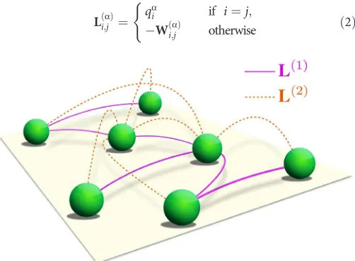
interactions among the units (see Fig. 1 for a schematic illustration of the case ofM= 2 layers andN= 7 nodes). Note that in our setting, the nodes interacting in each layer are literally the same elements. Nodei in layer 1 is precisely the same node as nodeiin layer 2, 3, orM. This contrasts with other works in which there is a one-to-one correspon-dence between nodes in different layers, but these represent poten-tially different states. The weights of the connections between nodes in layera(a= 1,…,M) are given by the elements of the matrixW(a)_, which is, therefore, the adjacency matrix of a weighted graph. The sum

qa i ¼

∑

N

j¼1W

ðaÞ

i;j ði¼1;…;NÞ

of the weights of all the interactions of nodeiin layerais the strength of the node in that layer.

Regarding the dynamics, each node represents ad-dimensional dy-namical system. Thus, the state of nodeiis described by a vectorx_iwith dcomponents. The local dynamics of the nodes is captured by a set of differential equations of the form

x˙_i¼FðxiÞ

where the dot indicates time derivative andFis an arbitraryC1-vector field. Similarly, the interaction in layerais described by a continuous and differentiable vector fieldH_a(generally different from layer to layer), possibly weighted by a layer-dependent coupling constantsa. We assume that the interactions between nodeiand nodejare diffusive, that is, for each layer in which they are connected, their coupling de-pends on the difference betweenH_aevaluated onxjandxi. Then, the dynamics of the whole system is described by the following set of equations

x˙_i¼FðxiÞ

∑

∑

N

j¼1L

ðaÞ

i;j HaðxjÞ ð1Þ

whereL(a)is the graph Laplacian of layera, whose elements are

LðaÞ i;j ¼

qa

i if i¼j; WðaÞ

i;j otherwise (

ð2Þ

Note that our treatment of this setting is valid for all possible choices of

FandH_a, so long as they areC1, and for any particular undirected struc-ture of the layers. This stands in contrast to other approaches to the study of the same equation set (1) proposed in previous works (and termed as dynamical hypernetworks), which, although based on ingenious techni-ques such as simultaneous block diagonalization, can be applied only to special cases [such as commuting Laplacians, unweighted and fully connected layers, and nondiffusive coupling (74)] or cannot guarantee to always provide a satisfactory solution (75).

Stability of complete synchronization in networks with multiple layers of interactions

We are interested in assessing the stability of synchronized states, which means determining whether a system eventually returns to the synchronized solution after a perturbation. For further details of the following derivations, we refer to Materials and Methods.

First, note that because Laplacians are zero-row-sum matrices, they all have a null eigenvalue, with corresponding eigenvectorN−1/2 (1, 1,…, 1)T, where T indicates transposition. This means that the gen-eral system of equations (1) always admits an invariant solutionS≡ {x_i(t) =s(t),∀i= 1, 2,…,N}, which defines the complete synchroni-zation manifold inℝdN.

Because one does not need a very strong forcing to destroy synchro-nization in an unstable state, we aim at predicting the behavior of the system when the perturbation is small. First, we linearize Eq. 1 around the synchronized manifoldSby obtaining the equations ruling the evolution of the local and global synchronization errorsdxi≡xi−s

anddX≡dx1,dx2,…,dxN)T

dX˙¼ 1⊗JFðsÞ

∑

M

a¼1saL

ðaÞ_⊗JH aðsÞ

!

dX ð3Þ

where1is theN-dimensional identity matrix,⨂denotes the Kronecker product, andJis the Jacobian operator.

Second, we spectrally decomposedXin the equation above and proj-ect it onto the basis defined by the eigenvproj-ectors of one of the layers. The particular choice of layer is completely arbitrary because the eigenvec-tors of the Laplacians of each layer formMequivalent bases ofℝN. In the following, to fix the ideas, we operate this projection onto the eigenvectors ofL(1). With some algebra, the system of equations 3 can then be expressed as

h˙ j¼

JFðsÞ s1lð 1Þ

j JH1ðsÞ

hjþ

∑

∑

N

k¼2

∑

r¼2l

ðaÞ

r G

ðaÞ r;kG

ðaÞ

r;jJHaðsÞhk ð4Þ

forj= 2,…,N, wherehjis the vector coefficient of the eigendecomposi-tion ofdX, andlðraÞis therth eigenvalue of the Laplacian of layera, sorted in a nondecreasing order; we have putGðaÞ ≡VðaÞ

T

Vð1Þ_{, in whichV}(a) indicates the matrix of eigenvectors of the Laplacian of layera. Note that to obtain this result, one must ensure that the Laplacian eigen-vectors of each layer are orthonormal, a choice that is always possible because all the Laplacians are real symmetric matrices. Thus, the sums run from 2 rather than 1 because the first eigenvalue of the La-placian, corresponding tor= 1, is always 0 for all layers, and the first eigenvector, to which all others are orthogonal, is common to all layers. Fig. 1. Schematic representation of a network with two layers of interaction.The

two layers (corresponding here to solid violet and dashed orange links) are made of links of different types for the same nodes, such as different means of transport be-tween two cities or chemical and electric connections bebe-tween neurons. Note that the layers are fully independent, in that they are described by two different LaplaciansL(1) andL(2)_{, so that the presence of a connection between two nodes in one layer does not} affect their connection status in the other.

on November 17, 2016

http://advances.sciencemag.org/

Equation 4 is notable in that it includes previous results about systems with commuting Laplacians as a special case. If the Laplacians commute, they can be simultaneously diagonalized by a common basis of eigenvectors. Thus, in this case,V(a)=V(1)≡Vfor alla. In turn, this implies thatГ(a)=1for alla, and Eq. 4 becomes

h˙_{j¼JFðsÞ s1l}ð1Þ j JH1ðsÞ

hjþ

∑

∑

N

k¼2

∑

r¼2l

ðaÞ

r dr;kdr;jJHaðsÞhk ¼JFðsÞ

∑

M

a¼1sal

ðaÞ j JHaðsÞ

hj

recovering anM-parameter variational form as in (74).

Note that the stability of the synchronized state is completely spe-cified by the maximum conditional Lyapunov exponentL, corresponding to the variation of the norm ofW≡(h2,…,hN). BecauseWwill evolve

on average as |W|(t)~exp(Lt), the fully synchronized state will be stable against small perturbations only ifL< 0.

Case study: Networks of Rössler oscillators

To illustrate the predictive power of the framework described above, we apply it to a network of identical Rössler oscillators, with two layers of connections. Note that our method is fully general, and it can be applied to systems composed by any number of layers and containing oscillators of any dimensionalityd. The particular choice ofM= 2 andd= 3 for our example allows us to study a complex phenomenology while retaining ease of illustration. The dynamics of the Rössler oscillators is described byx˙_{¼ ðyz;xþay;bþ ðxcÞzÞ}T

, where we have putx≡x1,y≡ x2, and z≡x3. The parameters are fixed to the valuesa= 0.2,b= 0.2, and c= 9, which ensure that the local dynamics of each node is chaotic.

Considering each layer of connections individually, it is known that the choice of the functionH allows (for an ensemble of net-worked Rössler oscillators) the selection of one of the three classes of stability (see Materials and Methods for more details), which are (i)H(x) = (0, 0,z), for which synchronization is always unstable; (ii)H(x) = (0,y, 0), for which synchronization is stable only for

sala2<0:1445;

(iii)H(x) = (x, 0, 0) for which synchronization is stable only for 0:181₌

la 2 <sa<

4:615₌

la N.

Because of the double layer structure, one can now combine together different classes of stability in the two layers, studying how one affects the other and identifying new stability conditions arising from the different choices. In the following, we consider three combi-nations, namely

Case 1:layer 1 in class I and layer 2 in class II, that is,H1(x) = (0, 0,z) andH2(x) = (0,y, 0);

Case 2:layer 1 in class I and layer 2 in class III, that is,H1(x) = (0, 0,z) andH2(x) = (x, 0, 0);

Case 3:layer 1 in class II and layer 2 in class III, that is,H1(x) = (0,y, 0) andH2(x) = (x, 0, 0).

As for the choices of the LaplaciansL(1,2), we consider three pos-sible combinations: (i) both layers as Erdős-Rényi networks of equal mean degree (ER-ER); (ii) both layers as scale-free networks with power-law exponent 3 (SF-SF); and (iii) layer 1 as an Erdős-Rényi network and layer 2 as a scale-free network (ER-SF). In all cases, the graphs are generated using the algorithm of Gómez-Gardeñes and Moreno (76), which allows a continuous interpolation between scale-free and Erdős-Rényi structures (see Materials and Methods

for details). Therefore, in the following, we will consider nine possible scenarios, that is, the three combinations of stability classes for each of the three combinations of layer structures.

Case 1.

Rewriting the system of equations (4) explicitly for each component of hj, we obtain here

h˙_j

1 ¼ hj2hj3 ð5Þ

h˙

j1 þ0:2hj

2 s2

∑

N

k¼2

∑

r¼2l

ð2Þ

r Gr;kGr;jhk2 ð6Þ

h˙_j

3 ¼s3hj₁þ ðs19Þhj₃s1l

ð1Þ

j hj3 ð7Þ

from which the maximum Lyapunov exponent can be numerically calculated. As shown in the top panel of Fig. 2, we observe that for ER-ER topologies, the first layer is dominated by the second because the stability region of the whole system appears to be almost independent ofs1, disregarding a slight increase of the critical value ofs2ass1increases. This demonstrates the ability of class II systems to control the instabilities inherent to systems in class I. This result appears to be robust with respect to the choice of underlying structures because qualitatively similar results are obtained for SF-SF, ER-SF, and SF-ER topologies (fig. S1).

Fig. 2. Maximum Lyapunov exponent for ER-ER topologies in case 1 (top panel) and case 2 (bottom panel).The darker blue lines mark the points in the (s1,s2) space whereLvanishes, whereas the striped lines indicate the critical values ofs2if layer 2 is considered in isolation (or, equivalently, ifs1= 0).

on November 17, 2016

http://advances.sciencemag.org/

Case 2.

For case 2, the system of equations (4) reads

h˙

j1 ¼ hj2hj3s2

∑

N

k¼2

∑

r¼2l

ð2Þ

r Gr;kGr;jhk1 ð8Þ

h˙

j2¼hj₁þ0:2hj2 ð9Þ

h˙_j

3 ¼s3hj₁þ ðs19Þhj₃s1l

ð1Þ

j hj3 ð10Þ

As shown in the bottom panel of Fig. 2, also in this case, the second layer strongly dominates the whole system because the overall stability window is almost independent from the value ofs1. This result, together with that obtained for case 1, suggests that class I systems, although intrinsically preventing synchronization, are easily controlla-ble by both class II and class III systems, even though, analogous to case 1, we observe a slight widening of the stability window for increasing values ofs1. Again, the results are almost independent from the choice of the underlying topologies (fig. S2).

Case 3.

Finally, for case 3, equations (4) become

h˙

j1 ¼ hj2hj3s2

∑

N

k¼2

∑

r¼2l

ð2Þ

r Gr;kGr;jhk1 ð11Þ

h˙

j2 ¼hj1þ0:2hj2s1l

ð1Þ

j hj2 ð12Þ

h˙

j3 ¼s3hj1þ ðs19Þhj3 ð13Þ

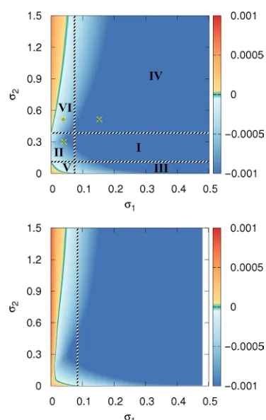
Here, the system reveals its most striking features. In particular, for ER-ER topologies (see top panel of Fig. 3), we observe six different regions, identified in the figure by Roman numerals. In region I, syn-chronization is stable in both layers taken individually (or, equivalent-ly, for eithers1= 0 ors2= 0), and the full bilayered network is also stable. Regions II, III, and IV correspond to scenarios qualitatively sim-ilar to the ones seen previously, that is, where stability properties of one layer dominate over those of the other. Finally, regions V and VI are the most important because within them, one finds effects that are genuinely arising from the multilayered nature of the interactions. In these regions, both layers are individually unstable, and synchronization would not be observed at all for eithers1= 0 ors2= 0. However, the emergence of a collective synchronous motion is remarkably ob-tained with a suitable tuning of the parameters. In these regions, it is therefore the simultaneous action of the two layers that induces stability.

Together, the results we obtained for the three cases indicate that a multilayer interaction topology enhances the stability of the synchro-nized state, even allowing for the possibility of stabilizing systems that are unstable when considered isolated.

Numerical validation

We validate the stability predictions derived from equations (4) by simulating the full nonlinear system of equations (1) for an ER-ER

topology in case 3, with three different choices of coupling constants

s1ands2. The three specific sets of coupling values (shown in the top panel of Fig. 3) correspond to situations in which either one or both layers are unstable when isolated but yield a stable synchronized state when coupled. More specifically, we have chosen (s1= 0.04,s2= 0.3), (s1 = 0.15, s2 = 0.5), and (s1 = 0.04,s2 = 0.5) corresponding to regions II, IV, and VI, respectively.

For all three cases, we run the simulations initially with the pres-ence of only the unstable layer, by setting eithers1= 0 ors2= 0 depend-ing on the set of coupldepend-ings considered. Note that for the third set of couplings (region VI), either layer can be the initially active one because both are unstable when isolated. After 100 integration steps, we then activate the other layer by setting its interaction strength to the (non-zero) value corresponding to the region for which we predicted a stable synchronized state. As the systems evolve, we monitor the evolution of the norm |W|(t) to evaluate the deviation from the synchronized solu-tion with time.

The results in Fig. 4 show that when only the unstable interaction layer is active, |W|(t) never vanishes. However, as soon as the other layer is switched on, the norm ofWundergoes a sudden change of behavior, starting an exponential decay toward 0. This confirms the prediction that the unstable behavior induced by each layer is compensated by the mutual presence of two interaction layers.

Qualitatively similar scenarios are observed in case 3 for SF-SF topol-ogies, as well as for ER-SF and SF-ER structures (fig. S3). Again, they Fig. 3. Maximum Lyapunov exponent in case 3 for ER-ER and SF-SF topologies (top and bottom panel, respectively).The darker blue lines mark the points in the (s1,s2) plane where the maximum Lyapunov exponent is 0, whereas the striped lines indicate the stability limits for thes1= 0 ands2= 0. The points marked in the top panel indicate the choices of coupling strengths used for the numerical validation of the model. Note that for SF networks in class III, the stability window disappears.

on November 17, 2016

http://advances.sciencemag.org/

confirm the correctness of the predictions, showing that in region I, layer 1 dominates over layer 2, and that in region II, overall stability can be induced even when both layers are unstable in isolation.

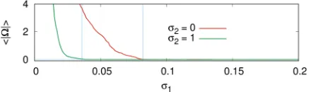
To provide an even stronger demonstration of the predictive power of our method, we simulate the full system for the ER-ER topology in case 3, fixing the value ofs2to 1 and varying the value ofs1from 0 to 0.2. Starting from an initial perturbed synchronized state, after a tran-sient of 100 time units, we measure the average of |W| over the next 20 integration steps. The results in Fig. 5 show agreement between the sim-ulations and the theoretical prediction (see Fig. 4). For values ofs1less than a critical value of approximately 0.04, the system never synchro-nizes. Conversely, whens1crosses the critical value, the system can reach a synchronized state. Repeating the simulation withs2= 0, one recovers the monoplex case. Also in this instance, we find agreement between theoretical prediction and simulation, with a critical coupling value of approximately 0.08.

DISCUSSION

The results shown above clearly illustrate the rich dynamical phenom-enology that emerges when the multilayer structure of real networked systems is taken into account. In an explicit example, we have observed that synchronization stability can be induced in unstable networked layers by coupling them with stable ones. In addition, we have shown that stability can be achieved even when all the layers of a complex sys-tem are unstable, if considered in isolation. This latter result constitutes a clear instance of an effect that is intrinsic to the true multilayer nature of the interactions among the dynamical units. Similarly, we expect that the opposite could also be observed, namely, that the synchronizability of a system decreases or even disappears when two individually syn-chronizable layers are combined.

On more general grounds, the theory developed here allows one to assess the stability of the synchronized state of coupled nonlinear dy-namical systems with multilayer interactions in a fully general setting. The system can have any arbitrary number of layers, and perhaps more importantly, the network structures of each layer can be fully in-dependent because we do not exploit any special structural or dynam-ical property to develop our theory. This way, our approach generalizes the celebrated MSF (30) to multilayer structures, retaining the general applicability of the original method. The complexity in the extra layers is reflected in the fact that the formalism yields a set of coupled linear dif-ferential equations (Eq. 4), rather than a single parametric variational

equation, which is recovered in the case of commuting Laplacians. This system of equations describes the evolution of a set ofd-dimensional vectors that encode the displacement of each dynamical system from the synchronized state. The solution of the system gives a necessary con-dition for stability: if the norm of these vectors vanishes in time, then the system gets progressively closer to synchronization, which is therefore stable; if, instead, the length of the vectors always remains greater than 0, then the synchronized state is unstable.

The generality of the method presented, which is applicable to any undirected structure, and its straightforward implementation for any choice ofC1dynamical setup pave the way for the exploration of syn-chronization properties on multilayer networks of arbitrary size and structure. Thus, we are confident that our work can be used in the de-sign of optimal multilayered synchronizable systems, a problem that has attracted much attention in monolayer complex networks (77–80). The straightforward nature of our formalism makes it suitable for efficient use together with successful techniques, such as the rewiring of links or the search for an optimal distribution of link weights, in the context of multilayer networks. In turn, these techniques may help in addressing the already mentioned question of the suppression of synchronization due to the interaction between layers, unveiling possible combinations of stable layers that, when interacting, suppress the dynamical coher-ence that they show in isolation. Also, we believe that the reliability of our method will provide aid to the highly current field of multiplex network controllability (26,81–84), enabling researchers to engineer control layers to drive the system dynamics toward a desired state.

In addition, several extensions of our work toward more general systems are possible. A particularly relevant one is the study of multilayer networks of heterogeneous oscillators, which have a rich phenomenology Fig. 4. Numerical validation of the stability analysis.The error of synchronization increases as long as the only active layer is the one predicted to be unstable. When the other layer is switched on, at time 100, the error of synchronization decays exponentially toward 0, as predicted by the model. With respect to Fig. 3, the top left panel corresponds to region II, where layer 1 is unstable and layer 2 is stable, and the interaction strengths used weres1= 0.04 ands2= 0.3. The bottom left panel corresponds to region IV, where layer 1 is stable and layer 2 is unstable, and the interaction strengths weres1= 0.15 ands2= 0.5. The top right and bottom right panels correspond to region VI, where both layers are unstable. The layer active from the beginning was layer 1 for the top right panel and layer 2 for the bottom right panel. In both cases, the interaction strengths weres1= 0.04 and

s2= 0.5.

Fig. 5. Identification of the critical points.For a system with ER-ER topology in case 3 and fixeds2= 1, the synchronization error never vanishes ifs1<sc≈0.04. Conversely, as soon ass1>sc, the system is again able to synchronize (green line). One recovers the monolayer case by imposings2= 0, for which similar results are found, with a critical coupling strength of approximately 0.08 (red line). Both results are in perfect agree-ment with the theoretical predictions (see Fig. 4).

on November 17, 2016

http://advances.sciencemag.org/

and whose synchronizability has been shown to depend on all the Laplacian eigenvalues (85) in a way similar to the results presented here. Relaxing the requirement of an undirected structure, our ap-proach can also be used to study directed networks. The graph Lapla-cians in this case are not necessarily diagonalizable, but a considerable amount of information can be still extracted from them using singular value decomposition. For example, it is already known that directed networks can be rewired to obtain an optimal distribution of in-degrees for synchronization (86). Further areas that we intend to ex-plore in future work are those of almost identical oscillators and almost identical layers, which can be approached using perturbative methods and constitute more research directions with even wider applicability.

Finally, as our method allows one to study the rich synchroniza-tion phenomenology of general multilayer networks, we believe that it will find application in technological, biological, and social systems where synchronization processes and multilayered interactions are at work. Some examples are coupled power grid and communication systems, some brain neuropathologies such as epilepsy, and the onset of coordinated social behavior when multiple interaction channels coexist. As mentioned above, these applications will demand further advances to include specific features such as the nonhomogeneity of interacting units or the possibility of directional interactions.

MATERIALS AND METHODS

Linearization around the synchronized solution

To linearize the system in Eq. 4 around the synchronization manifold, use the fact that for anyC1-vector fieldfwe can write

fðxÞ≈fðx0Þ þJfðx0Þ⋅ðxx0Þ

Using this relation, we can expandFandHaroundsin the sys-tem of equations 4 to obtain

dx˙i¼x˙is˙ ≈JFðsÞ⋅dxi

∑

a¼1saJHaðsÞ⋅

∑

j¼1L

ðaÞ

i;jdxj ð14Þ

Now, we use the Kronecker matrix product to decompose the equa-tion above into self-mixing and interacequa-tion terms and introduce the vectordX, to get the final system of equations 3. The system 3 can be rewritten by projectingdXonto the Laplacian eigenvectors of a layer. The choice of layer to carry out this projection is entirely arbitrary be-cause the Laplacian eigenvectors are always a basis ofℝN. Without the loss of generality, we choose layer 1 and ensure that the eigenvectors are orthonormal. We then define1dto be thed-dimensional identity matrix

and multiply Eq. 3 on the left by

Vð1ÞT_⊗1 d

Vð1ÞT

⊗1d

dX˙ ¼

Vð1ÞT_⊗1

d

1⊗JFðsÞ

∑

Vð1ÞT_⊗1 d

LðaÞ_⊗JH aðsÞ

dX

Now, we use the relation

ðM1⊗M2ÞðM3⊗M4Þ ¼ ðM1M3Þ⊗ðM2M4Þ ð15Þ

to obtain

Vð1ÞT_⊗1

d

dX:¼ Vð1Þ

T

⊗JFðsÞ s1Dð1ÞVð1Þ

T

⊗JH1ðsÞ

h i

dX

∑

Vð1ÞT_LðaÞ_⊗JH aðsÞdX

whereD(a)is the diagonal matrix of the eigenvalues of layera, and we have split the sum into the first term and the remainingM−1 terms. Left-multiply the first occurrence ofVð1ÞT_{in the right-hand side} by1, and right-multiplyFandH1by1d. Then, using again Eq. 15, it becomes

Vð1ÞT_⊗1

d

dX˙ ¼1⊗JFðsÞVð1Þ

T

⊗1d

s1Dð1Þ⊗JH1ðsÞ

Vð1ÞT_⊗1 d

dX

∑

ð1ÞT_LðaÞ_⊗JH aðsÞdX

Factor outVð1ÞT_⊗1 d

to get

Vð1ÞT_⊗1 d

dX: ¼

1⊗JFðsÞ s1Dð1Þ⊗JH1ðsÞ

Vð1ÞT_⊗1 d

dX

∑

M

a¼2saV

ð1ÞT_LðaÞ_⊗JH a

sdX

The relation

ðM1⊗M2Þ1_¼M

11⊗M21

implies that

Vð1Þ_⊗1

d

Vð1ÞT_⊗1

d

is themN-dimensional identity

matrix. Then, we left-multiply the lastdXby this expression, obtaining

Vð1ÞT_⊗1 d

dX˙ ¼

1⊗JFðsÞ s1Dð1Þ⊗JH1ðsÞ

Vð1ÞT_⊗1 d

dX

∑

ð1ÞT_LðaÞ_⊗JH

aðsÞ

Vð1Þ_⊗1

d

Vð1ÞT_⊗1

d

dX

Now, we define the vector-of-vectors

h≡Vð1ÞT ⊗1d

dX

Each component ofhis the projection of the global synchronization error vectordXonto the space spanned by the corresponding Laplacian eigenvector of layer 1. The first eigenvector, which defines the synchro-nization manifold, is common to all layers, and all other eigenvectors are orthogonal to it. Thus, the norm of the projection ofhover the space spanned by the lastN–1 eigenvectors is a measure of the synchroni-zation error in the directions transverse to the synchronisynchroni-zation

on November 17, 2016

http://advances.sciencemag.org/

manifold. Because of howhis built, this projection is just the vectorW, consisting of the lastN–1 components ofh. With this definition ofh, we left-multiplyL(a)by the identity expressed asVðaÞ_VðaÞT_{to obtain}

h˙ _{¼1⊗JFðsÞ s1D}ð1Þ_⊗JH1ðsÞh

∑

ð1ÞT_VðaÞ_DðaÞ_VðaÞT_Vð1Þ_⊗JH

a

sh

In this vector equation, the first part is purely variational because it consists of a block-diagonal matrix that multiplies the vector-of-vectors

h. However, the second part mixes different components ofh. This can be seen more easily expressing the vector equation as a system of equa-tions, one for each componentjofh.

To write this system, it is convenient to first defineGðaÞ ≡VðaÞTVð1Þ, then consider the nonvariational part. Its contribution to thejth component ofh˙ is given by the product of thejth row of blocks of the block-matrix multiplied byh. In turn, each element of this row of blocks consists of the corresponding element of thejth row of

GðaÞTDðaÞGðaÞmultiplied byJHa(s)

GðaÞ

T

DðaÞ_GðaÞ j;k¼

∑

N

r¼1G ðaÞT j;r lðraÞG

ðaÞ r;k

Summing over all the componentsh_kyields

h˙_{j¼JFðsÞ s1l}ð1Þ j JH1ðsÞ

hjþ

∑

∑

N

k¼2

∑

r¼2l

ðaÞ r Gð

aÞ

r;kG

ðaÞ

r;jJHaðsÞhk

which is Eq. 4. Note that the sums overrandkstart from 2 because the first eigenvalue is always 0, and the orthonormality of the eigenvectors guarantees that all the elements of the first column ofГ(a), except the first, are 0. Each matrixГ(a)effectively captures the alignment of the Laplacian eigenvectors of layerawith those of layer 1. If the eigenvectors for layera

are identical to those of layer 1, as it happens when the two Laplacians commute, thenГ(a)=1. One can generalize the definition ofГ(a)to con-sider any two layers, introducing the matricesXða;bÞ≡VðaÞTVðbÞ¼ GðaÞ_GðbÞT_{that can even be used to define a measureℓ}

Dof“dynamical distance”between two layersaandb

ℓD¼

∑

N

i¼2 "

∑

ð

ða;bÞ i;j

Þ

2#

ð

Þ

2

MSF and stability classes

A particular case of the treatment we considered above happens when M= 1. In this case, the second term on the right-hand side of Eq. 4 disappears, and the system takes the variational formh˙_i¼Kihi, where Ki≡JF(s)–sliJH(s) is an evolution kernel evaluated on the

synchro-nization manifold. Becausel1= 0, this equation separates the contri-bution parallel to the manifold, which reduces toh˙_1¼JFðsÞh1, from the otherN–1, which describe perturbations in the directions trans-verse to the manifold and which have to be damped for the synchro-nized state to be stable. Because the Jacobians ofFandHare evaluated on the synchronized state, the variational equations differ only in the eigenvaluesli. Thus, one can extract from each of them a set ofd

-conditional Lyapunov exponents, evaluated along the eigenmodes as-sociated toli. Puttingn≡sli, the parametrical behavior of the largest

of these exponentsL(n) defines the so-called MSF (30). If the network is undirected, then the spectrum of the Laplacian is real, and the MSF is a real function ofn. Crucially, for all possible choices ofFandH, the MSF of a network falls into one of three possible behavior classes, defined as follows (6)

class I:L(n) never intercepts thexaxis;

class II:L(n) intercepts thexaxis at a single point at somenc≥0;

class III: L(n) is a convex function with negative values within some window nc1<n<nc2; in general,nc1≥0, with the equality holding whenFsupports a periodic motion.

The elegance of the MSF formalism manifests itself at its finest for systems in class III, for which synchronization is stable only ifsl2>nc1 andslN<nc2hold simultaneously. This condition implieslN=_l2<nc2=_nc1. BecauselN=

l2is entirely determined by the network topology andnc2=nc1

depends only on the dynamical functionsFandH, one has a simple stability criterion in which structure and dynamics are decoupled.

Network generation

To generate the networks for our simulations, we used the algorithm described by Gómez-Gardeñes and Moreno (76), which creates a one-parameter family of complex networks with a tunable degree of heter-ogeneity. The algorithm works as follows: start from a fully connected network withm0nodes and a setccontainingN–m0isolated nodes. At each time step, select a new node fromcand link it to othermnodes, selected among all other nodes. The choice of the target nodes happens uniformly at random with probabilityaand following a preferential at-tachment rule with probability 1–a. Repeating these stepsN–m0 times, one obtains networks with the same number of nodes and links, whose structure interpolates between ER, fora= 1, and SF, fora= 0.

Numerical calculations

To compute the maximum Lyapunov exponent for a given pair of cou-pling strengthss1ands2, we first integrate a single Rössler oscillator from an initial state (0, 0, 0) for a transient timettrans, sufficient to reach the chaotic attractor. The integration is carried out using a fourth-order Runge-Kutta integrator with a time step of 5 × 10–3, for which we choose a transient timettrans= 300. Then, we integrate the systems for the perturbations (Eqs. 5 to 7, 8 to 10, and 11 to 13) using Euler’s method, again with a same time step of 5 × 10–3. The initial conditions are such that all components of all theh_jare1=pffiffiffiffiffiffiffiffiffiffiffiffiffiffiffiffiffiffi3ðN1Þ, makingWa unit vector. At the same time, we continue the integration of the single Rössler unit to provide fors1ands3, which appear in the perturbation equations. This process is repeated for 500 time windows, each with the duration of 1 unit (200 steps). After each windown, we compute the norm of the overall perturbation |W|(n) and rescale the components of theh_jso that at the start of the next time window, the norm ofW is again set to 1. Finally, when the integration is completed, we estimate the maximum Lyapunov exponent as

L¼ 1

500

∑

n¼1logðjWjðnÞÞ

SUPPLEMENTARY MATERIALS

Supplementary material for this article is available at http://advances.sciencemag.org/cgi/ content/full/2/11/e1601679/DC1

fig. S1. Maximum Lyapunov exponentLfor systems falling into case 1 (layer 1 in stability class I and layer 2 in stability class II) for SF-SF, ER-SF, and SF-ER topologies (left, center, and right panels, respectively).

on November 17, 2016

http://advances.sciencemag.org/

fig. S2. Maximum Lyapunov exponentLfor systems falling into case 2 (layer 1 in stability class I and layer 2 in stability class III) for SF-SF, ER-SF, and SF-ER topologies (left, center, and right panels, respectively).

fig. S3. Maximum Lyapunov exponentLfor systems falling into case 3 (layer 1 in stability class II and layer 2 in stability class III) for ER-SF and SF-ER topologies (left and right panels, respectively).

REFERENCES AND NOTES

1. S. H. Strogatz, Exploring complex networks.Nature410, 268–276 (2001).

2. R. Albert, A.-L. Barabási, Statistical mechanics of complex networks.Rev. Mod. Phys.74, 47–97 (2002).

3. M. E. J.Newman, The structure and function of complex networks.SIAM Rev. Soc. Ind. Appl. Math.45, 167–256 (2003).

4. S. N. Dorogovtsev, J. F. F. Mendes,Evolution of Networks: From Biological Nets to the Internet and WWW(Oxford Univ. Press, 2003).

5. E. Ben-Naim, H. Frauenfelder, Z. Toroczkai,Complex Networks (Lecture Notes in Physics) (Springer, 2004), vol. 650.

6. S. Boccaletti, V. Latora, Y. Moreno, M. Chavez, D.-U. Hwang, Complex networks: Structure and dynamics.Phys. Rep.424, 175–308 (2006).

7. G. Caldarelli,Scale-free Networks: Complex Webs in Nature and Technology(Cambridge Univ. Press, 2007).

8. M. E. J. Newman,Networks: An Introduction. (Oxford Univ. Press, 2010).

9. R. Cohen, S. Havlin,Complex Networks: Structure, Robustness and Function(Cambridge Univ. Press, 2010).

10. D. Watts, S. H. Strogatz, Collective dynamics of“small-world”networks.Nature393, 440–442 (1998).

11. A.-L. Barabási, R. Albert, Emergence of scaling in random networks.Science286, 509–512 (1999).

12. S. N. Dorogovtsev, A. V. Goltsev, J. F. F. Mendes, Critical phenomena in complex networks. Rev. Mod. Phys.80, 1275–1335 (2008).

13. R. Guimerá, L. A. N. Amaral, Functional cartography of complex metabolic networks. Nature433, 895–900 (2005).

14. S. Fortunato, Community detection in graphs.Phys. Rep.486, 75–174 (2010). 15. C. I. Del Genio, T. House, Endemic infections are always possible on regular networks.

Phys. Rev. E88, 040801 (2013).

16. T. P. Peixoto, Hierarchical block structures and high-resolution model selection in large networks.Phys. Rev. X4, 011047 (2014).

17. O. Williams, C. I. Del Genio, Degree correlations in directed scale-free networks.PLOS ONE 9, e110121 (2014).

18. S. Treviño III, A. Nyberg, C. I. Del Genio, K. E. Bassler, Fast and accurate determination of modularity and its effect size.J. Stat. Mech.2015, P02003 (2015).

19. M. E. J. Newman, T. P. Peixoto, Generalized communities in networks.Phys. Rev. Lett.115, 088701 (2015).

20. A. Barrat, M. Barthélemy, A. Vespignani,Dynamical Processes on Complex Networks (Cambridge Univ. Press, 2008).

21. B. Barzel, A.-L. Barabási, Universality in network dynamics.Nat. Phys.9, 673–681 (2013). 22. J. Gao, B. Barzel, A.-L. Barabási, Universal resilience patterns in complex networks.Nature

530, 307–312 (2016).

23. C. Castellano, S. Fortunato, V. Loreto, Statistical physics of social dynamics.Rev. Mod. Phys. 81, 591–646 (2009).

24. R. Pastor-Satorras, C. Castellano, P. Van Mieghem, A. Vespignani, Epidemic processes in complex networks.Rev. Mod. Phys.87, 925–979 (2015).

25. S. Boccaletti, J. Kurths, G. Osipov, D. L. Valladares, C. S. Zhou, The synchronization of chaotic systems.Phys. Rep.366, 1–101 (2002).

26. Y.-Y. Liu, J.-J. Slotine, A.-L. Barabási, Controllability of complex networks.Nature473, 167–173 (2011).

27. A. Pikovsky, M. Rosenblum, J. Kurths,Synchronization: A Universal Concept in Nonlinear Sciences(Cambridge Univ. Press, 2003).

28. S. H. Strogatz,Sync: The Emerging Science of Spontaneous Order(Hyperion, 2003). 29. S. C. Manrubia, A. S. Mikhailov, D. H. Zanette,Emergence of Dynamical Order.

Synchronization Phenomena in Complex Systems(World Scientific, 2004).

30. L. M. Pecora, T. L. Carroll, Master stability functions for synchronized coupled systems. Phys. Rev. Lett.80, 2109–2112 (1998).

31. L. F. Lago-Fernández, R. Huerta, F. Corbacho, J. A. Sigüenza, Fast response and temporal coherent oscillations in small-world networks.Phys. Rev. Lett.84, 2758–2761 (2000). 32. M. Barahona, L. M. Pecora, Synchronization in small-world systems.Phys. Rev. Lett.89,

054101 (2002).

33. T. Nishikawa, A. E. Motter, Y.-C. Lai, F. C. Hoppensteadt, Heterogeneity in oscillator networks: Are smaller worlds easier to synchronize?Phys. Rev. Lett.91, 014101 (2003). 34. I. V. Belykh, V. N. Belykh, M. Hasler, Blinking model and synchronization in small-world

networks with a time-varying coupling.Physica D195, 188–206 (2004).

35. D.-U. Hwang, M. Chavez, A. Amann, S. Boccaletti, Synchronization in complex networks with age ordering.Phys. Rev. Lett.94, 138701 (2005).

36. M. Chavez, D.-U. Hwang, A. Amann, H. G. E. Hentschel, S. Boccaletti, Synchronization is enhanced in weighted complex networks.Phys. Rev. Lett.94, 218701 (2005). 37. A. E. Motter, C.-S. Zhou, J. Kurths, Enhancing complex-network synchronization.Europhys.

Lett.69, 334–337 (2005).

38. C. Zhou, A. E. Motter, J. Kurths, Universality in the synchronization of weighted random networks.Phys. Rev. Lett.96, 034101 (2006).

39. I. Lodato, S. Boccaletti, V. Latora, Synchronization properties of network motifs.EPL78, 28001 (2007).

40. J. Gómez-Gardeñes, S. Gómez, A. Arenas, Y. Moreno, Explosive synchronization transitions in scale-free networks.Phys. Rev. Lett.106, 128701 (2011).

41. S. Bilal, R. Ramaswamy, Synchronization and amplitude death in hypernetworks.Phys. Rev. E89, 062923 (2014).

42. C. I. del Genio, M. Romance, R. Criado, S. Boccaletti, Synchronization in dynamical networks with unconstrained structure switching.Phys. Rev. E Stat. Nonlin. Soft Matter Phys.92, 062819 (2015).

43. S. Boccaletti, G. Bianconi, R. Criado, C. I. del Genio, J. Gómez-Gardeñes, M. Romance, I. Sendiña-Nadal, Z. Wang, M. Zanin, The structure and dynamics of multilayer networks. Phys. Rep.544, 1–122 (2014).

44. M. Kivelä, A. Arenas, M. Barthélemy, J. P. Gleeson, Y. Moreno, M. A. Porter, Multilayer networks.J. Complex Netw.2, 203–271 (2014).

45. K.-M. Lee, B. Min, K.-I. Goh, Towards real-world complexity: An introduction to multiplex networks.Eur. Phys. J. B.88, 48 (2015).

46. G. Bianconi, Interdisciplinary and physics challenges of network theory.EPL111, 56001 (2015).

47. M. Szell, R. Lambiotte, S. Thurner, Multirelational organization of large-scale social networks in an online world.Proc. Natl. Acad. Sci. U.S.A.107, 13636–13641 (2010). 48. A. Cardillo, J. Gómez-Gardeñes, M. Zanin, M. Romance, D. Papo, F. del Pozo, S. Boccaletti,

Emergence of network features from multiplexity.Sci. Rep.3, 1344 (2013). 49. A. Halu, S. Mukherjee, G. Bianconi, Emergence of overlap in ensembles of spatial

multiplexes and statistical mechanics of spatial interacting network ensembles.Phys. Rev. E Stat. Nonlin. Soft Matter Phys.89, 012806 (2014).

50. B. M. Adhikari, A. Prasad, M. Dhamala, Time-delay-induced phase-transition to synchrony in coupled bursting neurons.Chaos21, 023116 (2011).

51. F. Radicchi, A. Arenas, Abrupt transition in the structural formation of interconnected networks.Nat. Phys.9, 717–720 (2013).

52. J. Gómez-Gardeñes, M. De Domenico, G. Gutiérrez, A. Arenas, S. Gómez, Layer–Layer competition in multiplex complex networks.Philos. Trans. A Math. Phys. Eng. Sci.373, 20150117 (2015).

53. S. V. Buldyrev, R. Parshani, G. Paul, H. E. Stanley, S. Havlin, Catastrophic cascade of failures in interdependent networks.Nature464, 1025–1028 (2010).

54. S.-W. Son, G. Bizhani, C. Christensen, P. Grassberger, M. Paczuski, Percolation theory on interdependent networks based on epidemic spreading.EPL97, 16006 (2012). 55. J. Gao, S. V. Buldyrev, H. E. Stanley, S. Havlin, Networks formed from interdependent

networks.Nat. Phys.8, 40–48 (2012).

56. G. Bianconi, S. N. Dorogovtsev, Multiple percolation transitions in a configuration model of a network of networks.Phys. Rev. E Stat. Nonlin. Soft Matter Phys.,89, 062814 (2014).

57. G. J. Baxter, D. Cellai, S. N. Dorogovtsev, A. V. Goltsev, J. F. F. Mendes, A unified approach to percolation processes on multiplex networks, inInterconnected Networks, A. Garas, Ed. (Springer International Publishing, 2016), pp.101–123.

58. A. Saumell-Mendiola, M. Serrano, M. Boguñá, Epidemic spreading on interconnected networks.Phys. Rev. E Stat. Nonlin. Soft Matter Phys.86, 026106 (2012).

59. C. Granell, S. Gómez, A. Arenas, Dynamical interplay between awareness and epidemic spreading in multiplex networks.Phys. Rev. Lett.111, 128701 (2013).

60. C. Buono, L. G. Alvarez-Zuzek, P. A. Macri, L. A. Braunstein, Epidemics in partially overlapped multiplex networks.PLOS ONE9, e92200 (2014).

61. J. Sanz, C.-Y. Xia, S. Meloni, Y. Moreno, Dynamics of interacting diseases.Phys. Rev. X4, 041005 (2014).

62. G. Menichetti, L. Dall’Asta, G. Bianconi, Control of multilayer networks.Sci. Rep.6, 20706 (2016).

63. J. Gómez-Gardeñes, I. Reinares, A. Arenas, L. M. Floría, Evolution of cooperation in multiplex networks.Sci. Rep.2, 620 (2012).

64. Z. Wang, A. Szolnoki, M. Perc, Rewarding evolutionary fitness with links between populations promotes cooperation.J. Theor. Biol.349, 50–56 (2014).

65. J. T. Matamalas, J. Poncela-Casasnovas, S. Gómez, A. Arenas, Strategical incoherence regulates cooperation in social dilemmas on multiplex networks.Sci. Rep.5, 9519 (2015). 66. Z. Wang, L. Wang, A. Szolnoki, M. Perc, Evolutionary games on multilayer networks:

A colloquium.Eur. Phys. J. B.88, 124 (2015)

67. S. Gómez, A. Díaz-Guilera, J. Gómez-Gardeñes, C. J. Pérez-Vicente, Y. Moreno, A. Arenas, Diffusion dynamics on multiplex networks.Phys. Rev. Lett.110, 028701 (2013).

on November 17, 2016

http://advances.sciencemag.org/

68. R. Albert, H. Jeong, A.-L. Barabási, Error and attack tolerance of complex networks.Nature 406, 378–382 (2000).

69. M. M. Danziger, L. M. Shekhtman, A. Bashan, Y. Berezin, S. Havlin, Vulnerability of interdependent networks and networks of networks, inInterconnected Networks, A. Garas, Ed. (Springer International Publishing, 2016), pp. 79–99.

70. J. Aguirre, R. Sevilla-Escoboza, R. Gutiérrez, D. Papo, J. M. Buldú, Synchronization of interconnected networks: The role of connector nodes.Phys. Rev. Lett.112, 248701 (2015).

71. X. Zhang, S. Boccaletti, S. Guan, Z. Liu, Explosive synchronization in adaptive and multilayer networks.Phys. Rev. Lett.114, 038701 (2015).

72. R. Sevilla-Escoboza, R. Gutiérrez, G. Huerta-Cuellar, S. Boccaletti, J. Gómez-Gardeñes, A. Arenas, J. M. Buldú, Enhancing the stability of the synchronization of multivariable coupled oscillators.Phys. Rev. E Stat. Nonlin. Soft Matter Phys.92, 032804 (2015). 73. L. V. Gambuzza, M. Frasca, J. Gómez-Gardeñes, Intra-layer synchronization in multiplex

networks.EPL110, 20010 (2015).

74. F. Sorrentino, Synchronization of hypernetworks of coupled dynamical systems.New J. Phys.14, 033035 (2012).

75. D. Irving, F. Sorrentino, Synchronization of dynamical hypernetworks: Dimensionality reduction through simultaneous block-diagonalization of matrices.Phys. Rev. E Stat. Nonlin. Soft Matter Phys.86, 056102 (2012).

76. J. Gómez-Gardeñes, Y. Moreno, From scale-free to Erdős-Rényi networks.Phys. Rev. E Stat. Nonlin. Soft Matter Phys.73, 056124 (2006).

77. L. Donetti, P. Hurtado, M. A. Muñoz, Entangled networks, synchronization, and optimal network topology.Phys. Rev. Lett.95, 188701 (2005).

78. T. Nishikawa, A. E. Motter, Synchronization is optimal in nondiagonalizable networks. Phys. Rev. E73, 065106 (2006).

79. C. Zhou, J. Kurths, Dynamical weights and enhanced synchronization in adaptive complex networks.Phys. Rev. Lett.96, 164102 (2006).

80. T. Nishikawa, A. E. Motter, Network synchronization landscape reveals compensatory structures, quantization, and the positive effect of negative interactions.Proc. Natl. Acad. Sci. U.S.A.107, 10342–10347 (2010).

81. T. Nepusz, T. Vicsek, Controlling edge dynamics in complex networks.Nat. Phys.8, 568–573 (2012).

82. J. Sun, A. E. Motter, Controllability transition and nonlocality in network control.Phys. Rev. Lett.110, 208701 (2013).

83. J. Gao, Y.-Y. Liu, R. M. D’Souza, A.-L. Barabási, Target control of complex networks.Nat. Commun.5, 5415 (2014).

84. P. S. Skardal, A. Arenas, Control of coupled oscillator networks with application to microgrid technologies.Sci. Adv.1, e1500339 (2015).

85. P. S. Skardal, D. Taylor, J. Sun, Optimal synchronization of complex networks.Phys. Rev. Lett.113, 144101 (2014).

86. P. S. Skardal, D. Taylor, J. Sun, Optimal synchronization of directed complex networks. Chaos26, 094807 (2016).

Acknowledgments:We thank A. Arenas and J. Buldú for interesting and fruitful discussions. Funding:The work of J.G.-G. was supported by the Spanish MINECO through grants FIS2012-38266-C02-01 and FIS2011-25167 and by the European AQ38 Union through FET Proactive Project MULTIPLEX (Multilevel Complex Networks and Systems) contract no. 317532. Author contributions:C.I.d.G. and S.B. developed the theory. S.B. designed the simulations. J.G.-G. implemented and carried out the simulations and analyzed the results. All authors wrote the manuscript.Competing interests:The authors declare they have no competing interests.Data and material availability:All data needed to evaluate the conclusions in the paper are present in the paper and/or the Supplementary Materials. Additional data related to this paper may be requested from the authors.

Submitted 20 July 2016 Accepted 13 October 2016 Published 16 November 2016 10.1126/sciadv.1601679

Citation:C. I. del Genio, J. Gómez-Gardeñes, I. Bonamassa, S. Boccaletti, Synchronization in networks with multiple interaction layers.Sci. Adv.2, e1601679 (2016).

on November 17, 2016

http://advances.sciencemag.org/

doi: 10.1126/sciadv.1601679 2016, 2:.

Sci Adv

Stefano Boccaletti (November 16, 2016)

this article is published is noted on the first page.

This article is publisher under a Creative Commons license. The specific license under which

article, including for commercial purposes, provided you give proper attribution.

licenses, you may freely distribute, adapt, or reuse the

CC BY

For articles published under

. here

Association for the Advancement of Science (AAAS). You may request permission by clicking for non-commerical purposes. Commercial use requires prior permission from the American

licenses, you may distribute, adapt, or reuse the article

CC BY-NC

For articles published under

http://advances.sciencemag.org. (This information is current as of November 17, 2016): The following resources related to this article are available online at

http://advances.sciencemag.org/content/2/11/e1601679.full

online version of this article at:

including high-resolution figures, can be found in the Updated information and services,

http://advances.sciencemag.org/content/suppl/2016/11/14/2.11.e1601679.DC1

can be found at: Supporting Online Material

http://advances.sciencemag.org/content/2/11/e1601679#BIBL

6 of which you can access for free at: cites 75 articles,

This article

trademark of AAAS

otherwise. AAAS is the exclusive licensee. The title Science Advances is a registered York Avenue NW, Washington, DC 20005. Copyright is held by the Authors unless stated published by the American Association for the Advancement of Science (AAAS), 1200 New

(ISSN 2375-2548) publishes new articles weekly. The journal is Science Advances

on November 17, 2016

http://advances.sciencemag.org/