Atomistic to continuum coupling

http://wrap.warwick.ac.uk/

Original citation:

Luskin, Mitchell and Ortner, Christoph. (2013) Atomistic-to-continuum coupling. Acta Numerica, Volume 22 . pp. 397-508. ISSN 0962-4929

Permanent WRAP url:

http://wrap.warwick.ac.uk/49698/

Copyright and reuse:

The Warwick Research Archive Portal (WRAP) makes this work by researchers of the University of Warwick available open access under the following conditions. Copyright © and all moral rights to the version of the paper presented here belong to the individual author(s) and/or other copyright owners. To the extent reasonable and practicable the material made available in WRAP has been checked for eligibility before being made available.

Copies of full items can be used for personal research or study, educational, or not-for-profit purposes without prior permission or charge. Provided that the authors, title and full bibliographic details are credited, a hyperlink and/or URL is given for the original metadata page and the content is not changed in any way.

Publisher’s statement:

Copyright © Cambridge University Press 2013

A note on versions:

The version presented in WRAP is the published version or, version of record, and may be cited as it appears here.

http://journals.cambridge.org/ANU

Additional services for

Acta Numerica:

Email alerts: Click here Subscriptions: Click here Commercial reprints: Click here Terms of use : Click here

Atomistic-to-continuum coupling

Mitchell Luskin and Christoph Ortner

Acta Numerica / Volume 22 / May 2013, pp 397 - 508

DOI: 10.1017/S0962492913000068, Published online: 02 April 2013

Link to this article: http://journals.cambridge.org/abstract_S0962492913000068

How to cite this article:

Mitchell Luskin and Christoph Ortner (2013). Atomistic-to-continuum coupling. Acta Numerica, 22, pp 397-508 doi:10.1017/S0962492913000068

Request Permissions : Click here

doi:10.1017/S0962492913000068 Printed in the United Kingdom

Atomistic-to-continuum coupling

Mitchell Luskin

School of Mathematics, University of Minnesota,

MN 55455, USA E-mail: luskin@umn.edu

Christoph Ortner

Mathematics Institute, University of Warwick, Coventry CV4 7AL, UK E-mail: c.ortner@warwick.ac.uk

Atomistic-to-continuum (a/c) coupling methods are a class of computational multiscale schemes that combine the accuracy of atomistic models with the efficiency of continuum elasticity. They are increasingly being utilized in ma-terials science to study the fundamental mechanisms of material failure such as crack propagation and plasticity, which are governed by the interaction between crystal defects and long-range elastic fields.

CONTENTS

1 Introduction 398

2 Atomistic-to-continuum Lennard-Jones NNN models 402 3 Atomistic simulation 422 4 Many-body finite-range atomistic-to-continuum coupling 431

5 Coarsening error 444

6 Consistency 446

7 Stability 463

8 A priori error estimates and computational cost 475

9 Extensions and open problems 487

A Proofs 493

B Inverse function theorem 499

C List of symbols 500

References 502

1. Introduction

Crystal defects such as grain boundaries, cracks, or dislocations play a cen-tral role in determining material behaviour, and their study represents a substantial component of materials science research. Molecular simulation provides a unique way to study complex material behaviour at the nanoscale, in particular how defects affect macroscopic processes such as elasticity, plasticity, and fracture.

The key difficulty in atomistic simulation is that crystal defects affect elastic fields far beyond their immediate atomic neighbourhood; that is, they give rise to strongly coupled multiscale problems. Computational materials scientists therefore face a compromise between inaccurate atomistic models and inaccurate representations of the crystal environment.

Since defects occupy only a small proportion of bulk crystals, one may attempt to model the elastic fields using more efficient models of continuum elasticity. This idea naturally leads to the construction of concurrent cou-plings between atomistic descriptions of defect cores and continuum elastic-ity descriptions of the elastic fields. We henceforth refer to techniques of this kind as atomistic-to-continuum coupling methods, or simply a/c methods. By employing coarse discretizations (e.g., finite elements) of the continuum elasticity model they achieve a considerable reduction in computational cost compared to full atomistic descriptions, and potentially circumvent the com-promise between model accuracy and system size.

a/c coupling scheme, and to evaluate the relative accuracy and efficiency of different types of a/c coupling. Our aim is to provide a reference that will motivate further work by applied mathematicians in general and nu-merical analysts in particular, and a transfer of modern nunu-merical analysis methodologies.

During the past century, physicists and engineers have developed the sub-ject of micromechanics to give a fundamental understanding to the mech-anism of material failure. The building blocks of micromechanics are the nucleation and movement of point, line, and surface defects and their long-range elastic interactions. These mechanisms were first verified against macroscopic experiments and then more recently against experiments at the nanoscale. Computational micromechanics has begun to extend the predictive scope of theoretical micromechanics, but mathematical theory able to assess the accuracy and efficiency of multiscale methods is needed for computational micromechanics to reach its full potential. We hope that this article will help to nucleate a much wider research effort to establish rigorous mathematical underpinnings for (computational) micromechanics.

1.1. Brief history

Remarkably, the history of atomistic-to-continuum multiscale methods be-gins at a time when the existence of atoms had not even been confirmed: Cauchy (1882), in a search for simplified stress–strain relations for contin-uum elasticity, postulated a pair interaction law between atoms arranged in a crystalline structure and derived symmetry relations for the elastic constants known asCauchy relations. Various similar connections between atomistic and continuum descriptions of matter were used in solid state physics throughout the twentieth century: see Born and Huang (1954) for a standard reference.

As the critical role of crystal defects became more widely understood, the first ideas of a/c coupling emerged. Numerous authors in the 1950s and 1960s employed continuum linear elasticity to obtain boundary conditions for an atomistic simulation of a defect core; see Kanzaki (1957) for an early example. Eventually, it was recognized that, conversely, the defect core also provides boundary conditions for the elastic field and hence the two descriptions were coupled to interact concurrently. The first instance of such a method that we are aware of was developed by Sinclair (1971), and we may consider this as the first a/c coupling scheme.

The first occurrences of a/c couplings employing finite element methodol-ogy to discretize the continuum model can be found in the works of Baskes, Melius and Wilson (1981), Mullins and Dokainish (1982), Fischmeisteret al.

of the Cauchy–Born model by Tadmor, Ortiz and Phillips (1996). The latter reference coined the popular term ‘quasicontinuum method’.

By this point, it had became widely understood that the interface (or handshake region) treatment was critical in the construction of accurate and reliable a/c couplings. Various new ideas were put forward, most prominently, the iterative ghost force correction method (Shenoy et al.

1999), force-based a/c coupling (Curtin and Miller 2003), blending schemes (Xiao and Belytschko 2004), and the quasi-nonlocal coupling (Shimokawa, Mortensen, Schiøtz and Jacobsen 2004).

The first numerical analysis contributions to the field of a/c coupling are the works of Lin (2003) and Blanc, Le Bris and Legoll (2005). The first analyses that focused on the effect of different a/c interface treatments on the global error can be found in Dobson and Luskin (2009a, 2009b) and Ming and Yang (2009). The nonlinear analysis framework that we use in this article was introduced in Ortner and S¨uli (2008) and Ortner (2011). From here on, the numerical analysis of a/c coupling has turned into a rapidly developing field. We will introduce some of the key ideas and survey the various contributions throughout the remainder of this paper.

1.2. Outline and reading guide

This article is essentially divided into two parts, which can be read indepen-dently. The first part, which comprises only Section 2, gives a rapid formal introduction to the main ideas in the simplest possible non-trivial setting of second neighbour Lennard-Jones interaction in one dimension. Already in this simple setting, many interesting aspect of a/c coupling can be dis-cussed. Section 2 is intended to provide a first glimpse of the subject, or as the basis of a short series of lectures, or simply for readers who prefer explicit computations in a relatively simple setting over general mathemat-ical structure and rigorous proofs. We summarize the main conclusions of Section 2 in Table 2.1.

In the remainder of the article we develop a complete theory of a/c cou-pling for static defect computations in 1D. Although a theory of a/c coucou-pling in 2D/3D is now beginning to emerge, there are too many gaps and open questions to present a unified picture. Instead, we have chosen to present the 1D theory in a way that allows us to discuss existing generalizations to 2D/3D, as well as point out gaps. Moreover, with the exception of the reflection method introduced in Section 4.5, we only analyse a/c couplings whose formulations translate verbatim to 2D/3D.

Atomistic-to-continuum couplings can simply be considered as an approxi-mation scheme for this atomistic model. To analyse the errors committed, we employ the two fundamental concepts of numerical analysis: consistency and stability(see Section 4.7 for a formal outline of the approximation error analysis). The two central sections in this article are Section 6, where we establish the consistency of a/c couplings, and Section 7, where we estab-lish their stability. These results are then combined and further refined in Section 8 intoa priori error estimates in terms of computational cost.

The consistency error estimates and thea priorierror estimates are sum-marized, respectively, in Tables 6.1 and 8.1.

Throughout the article, we discuss relevant background literature, ex-isting extensions of our presentation to 2D/3D, and open problems. In addition, in Section 9 we give brief summaries of various extensions of the presentation in this article and a discussion of pressing open problems.

1.3. Omissions

No review article on a field of research as rich as a/c coupling can be com-plete. Our choice of topics reflects our personal view on the most important generic ideas in a/c coupling: the Cauchy–Born approximation, ghost forces at local/nonlocal model interfaces, ghost force reduction via blending, ghost force removal by conservative interface corrections, and force-based (non-conservative) a/c coupling.

We exclude many variants of how to combine these ingredients into practi-cal a/c coupling schemes, as well as other classes of a/c multispracti-cale methods. The analytical tools developed in this article for a/c coupling can poten-tially provide a framework for analysing these omitted methods, and we would consider the writing of this article a success if it motivates new re-search in this direction. The reader should refer to Section 9 for further discussions.

1.4. Notation

Notation is introduced throughout the manuscript where it is natural to do so. We have included a table of symbols in Appendix C.

Here, we merely mention that our notation forp and Lp norms is stan-dard. For a functionv with discrete domain X and A ⊂ X, we define

vp_(A) :=

(_ξ∈A|v(ξ)|p)1/p, 1≤p <∞, sup_ξ∈A|v(ξ)|, p=∞.

If we omit the domain in vp, then the norm is computed on the entire

Analogously, for a Lebesgue-measurable functionv:X→R, whereX ⊂ Ris measurable, and forA⊂X, we define

vLp_(A):=

(_A|v(x)|pdx)1/p, 1≤p <∞, ess sup_x∈A|v(x)|, p=∞.

If we omit the domain in vLp, then the norm is computed on the entire

domain of definitionX.

When we writef g,we mean that there exists a constantC >0, inde-pendent of the solution and approximation parameters, such thatf ≤Cg.

2. Atomistic-to-continuum Lennard-Jones next-nearest neighbour models

In this section, we offer a brief introduction in the simplest non-trivial set-ting, the Lennard-Jones next-nearest neighbour model. For the sake of simplicity of presentation, we keep this section entirely formal. Except where stated otherwise, all statements can be made rigorous. In fact, we present rigorous proofs for most of the statements in greater generality in subsequent sections.

We emphasize from the outset that the 1D Lennard-Jones model hides many fundamental issues one has to face when dealing with general many-body and 2D/3D situations, which are not merely of a technical nature. We will occasionally comment on such discrepancies.

2.1. The atomistic Lennard-Jones next-nearest neighbour model

We consider an infinite atomistic chain, indexed byZ. A displacement of the chain is a mapu:Z→R,where we will assume thatu(ξ)→0 as|ξ| → ∞. The reference lattice is AZ, where A > 0 is a macroscopic stretch, so the corresponding deformation of the atomistic chain is given by the mapping

ξ∈Ztoy(ξ) :=Aξ+u(ξ).We normally assume thatyis strictly increasing, that is,y(ξ)−y(ξ−1)>0,and henceu(ξ)−u(ξ−1)>−1 for allξ.

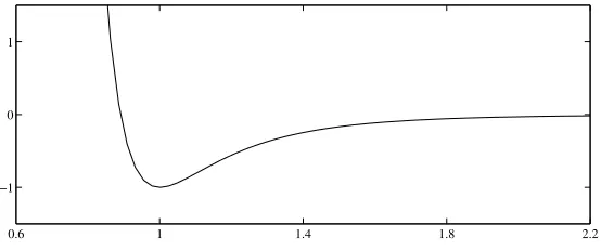
We assume in this introductory section that first and second neighbours interact via the Lennard-Jones potential φ(r) = r−12−2r−6 (or a similar pair potential): see Figure 2.1. The energy of a displacementucan then be written as

Ea(u) := ξ∈Z

φy(ξ)−y(ξ−1)+φy(ξ+ 1)−y(ξ−1)

= ξ∈Z

φ(A+u_ξ) +φ(2A+u_ξ+u_ξ+1)

= ξ∈Z

φ1(u_ξ) +φ2(u_ξ+u_ξ+1),

0.6 1 1.4 1.8 2.2 −1

0 1

Figure 2.1. The Lennard-Jones potential.

ξ _{ξ+ 1ξ+ 2} ξ−2ξ−1

Figure 2.2. Interactions in a 1D second-neighbour model.

where

φi(s) :=φ(iA+s) and uξ:=u(ξ)−u(ξ−1)

(and henceu_ξ+u_ξ+1=u(ξ+ 1)−u(ξ−1)).

More realistic molecular interactions are usually modelled via many-body potentials (see Section 3.2). Hence, to appreciate certain design decisions in coarse-graining schemes, it is important that we sometimes writeEa in a form that can be generalized:

Ea_{(u) =}

ξ∈Z

Φa_ξ(u), where the atomistic site energy is (2.2)

Φa_ξ(u) := 1₂φ1(uξ) +φ1(uξ+1) +φ2(uξ−1+uξ) +φ2(uξ+1+uξ+2)

.

See Figure 2.2 for an illustration.

We will see in Section 3.2 that if we assume without loss of generality thatφ1(0) +φ2(0) = 0, thenEa is well-defined on a suitable function space

of displacements. We will assume in this section that all displacement trial and test functions belong to this space, which we will later denote byU.

For simplicity, we consider only dead load external forces throughout this article. Letf :Z→Rwithf(ξ)→0 as|ξ| → ∞. Then we seek a solution of

ua_{∈arg minE}a_{(u)− f, u}

Z, (2.3)

equation

δEa(ua), v=f, v_Z for all v, where (2.4) δEa(u), v=

ξ∈Z

φ₁(u_ξ)v_ξ +φ₂(u_ξ+u_ξ+1)(v_ξ+v_ξ+1)

= ξ∈Z

φ

1(uξ) +φ2(uξ−1+uξ) +φ2(uξ+uξ+1)vξ (2.5)

= ξ∈Z

Sa_ξ(u)v_ξ

for anatomistic stress Sa_ξ(u) defined by

Sa_ξ(u) :=φ₁(u_ξ) +φ₂(u_ξ−1+u_ξ) +φ₂(u_ξ+u_ξ+1). (2.6)

Remark 2.1. We think of (2.3) as the ‘thermodynamic limit’ (at zero temperature) of a chain of N atoms as N → ∞. The advantage over the ‘scaling limit’, in which one would let the atomic spacing tend to zero, is that the thermodynamic limit keeps the atomistic detail we are interested in, but removes the dependence on boundary conditions. Intuitively, we can simply think of (2.3) as an infinite chain approximation of a large but finite chain.

2.2. The Cauchy–Born approximation

To approximate the atomistic description, we wish to model the infinite chainZusing a continuum elasticity model with an energy functional of the form

Ec(u) =

RW(∇u) dx, (2.7)

whereW : (−1,∞) →R is a suitable strain energy function and u is now defined forx ∈R. Interpreting∇u as a homogeneous strain applied to the infinite crystalZ, and henceW(∇u) as the resulting energy per unit volume corresponding to the atomistic model (2.1), we obtain the Cauchy–Born strain energy density function

W(F) :=φ1(F) +φ2(2F). (2.8)

We note thatW(0) = 0 sinceφ1(0)+φ2(0) = 0,and (2.7) is thus well-defined

on a suitable function space of displacements that decay at infinity.

In the remainder of Section 2, we consider a finite element Cauchy–Born model, taking the atomistic chain as the set of nodes; that is, for discrete displacementsu:Z→R, we (re-)define

Ec(u) = ξ∈Z

which is in fact equivalent to (2.7) when u(x) : R → R is the continuous piecewise linear interpolant ofu:Z→R.

For this discretized Cauchy–Born model, we seek

uc∈arg minEc(u)− f, u_Z. (2.9)

Solutions of (2.9) solve the Euler–Lagrange equation

δEc_(uc_{), v=f, v}

Z for all v, where (2.10)

δEc_{(u), v=}

ξ∈Z

∂_FW(u_ξ)v_ξ, (2.11)

where∂_FW(u_ξ) is the 1D variant of the first Piola–Kirchhoff stress tensor. Suppose thatEc is uniformlystableon{sua+ (1−s)uc|0≤s≤1}in the sense that there existsγ >0 such that

γv2

2 ≤ δ2Ec(sua+ (1−s)uc)v, v for allv, 0≤s≤1 (2.12)

(see (2.16) for an analysis of stability of the reference state and Section 7 for a rigorous general analysis). We then obtain

γ(ua−uc)22 ≤ 1

0 δ

2_Ec_(sua_{+ (1−s)u}c_{) ds(u}a_−uc_{), u}a_−uc

=

1

0

d dsδE

c_(sua_{+ (1−s)u}c_{) ds , u}a_−uc

=δEc(ua)−δEc(uc), ua−uc

=δEc(ua)−δEa(ua), ua−uc,

where, in the last equality, we have employed (2.4) and (2.10) (Galerkin orthogonality). Dividing through byγ(ua−uc)2, we arrive at

(ua−uc)2 ≤γ−1 sup

v

2=1

δEc_(ua_)−δEa_(ua_{), v, (2.13)}

which is reminiscent of the ‘variational crimes’ (or, simply,consistency er-ror) studied in the finite element literature. We call the right-hand side of (2.13) themodelling error of the Cauchy–Born model.

Applying (2.5) and (2.11), we obtain

δEc(u)−δEa(u), v= ξ∈Z

∂_FW(u_ξ)−Sa_ξ(u)v_ξ

= ξ∈Z

2φ₂(2u_ξ)−φ₂(u_ξ+u_ξ+1)−φ₂(u_ξ−1+u_ξ)v_ξ.

estimate

δEc(u)−δEa(u), vu2+u24

v2, (2.14)

whereu_ξ :=u_ξ+1−u_ξandu_ξ :=u_ξ−u_ξ−1.Inserting this result into (2.13), we obtain the second-order error estimate

(ua−uc)2 (ua)2+(ua)24. (2.15)

This error estimate states that, if (ua)_ξ varies slowly relative to the atomic spacing, then the Cauchy–Born solution is a good approximation to the atomistic solution. A fully analogous result, valid in 2D/3D and for general many-body interactions, is given by Ortner and Theil (2013); see also E and Ming (2007) and Makridakis and S¨uli (2013) for related results in this direction.

Remark 2.2 (scaling). All of the formulations and results in this paper can be given from the point of view of the scaling limit rather than the

thermodynamic limit as described in Remark 2.1. For example, rescaling space through ξ ξ and u(ξ) u(ξ), where is the atomic spacing, gives the second-order estimate

(ua−uc)2

2_(ua₎

2

+

2_(ua₎2

4

,

wherevp := (

ξ∈Z|vξ|p)1/p.

We prefer to use atomic units since they enable us to focus on the atom-istic details, as in applications the geometry of the defect core is a quantity of interest.

Stability of atomistic and Cauchy–Born models

In the formal error analysis above, we have seen how the stability, that is, positive-definiteness of the Hessian of the approximate model, comes into play. To indicate why we would expect (2.12) to hold, we briefly analyse the atomistic and Cauchy–Born Hessians at the reference state.

The Cauchy–Born and atomistic Hessians are, respectively, given by

δ2_Ec_{(0)v, v=W(0)}

ξ∈Z

|v

ξ|2, (2.16)

δ2_Ea_{(0)v, v=φ} 1(0)

ξ∈Z

|v

ξ|2+φ2(0)

ξ∈Z v

ξ+vξ+12.

Noting thatW(0) =φ₁(0)+4φ₂(0) and applying the parallelogram identity

v

ξ+vξ+12 = 2|vξ|2+ 2|vξ+1|2− |vξ|2 (2.17) (recall thatv_ξ=v_ξ+1−v_ξ), we observe that

δ2Ea(0)v, v=δ2Ec(0)v, v−φ₂(0) ξ∈Z

ξ

∇u(ξ)

defect core elastic bulk elastic bulk

Figure 2.3. 1D analogy of a crystal defect: the deformation field varies rapidly in the defect core but is ‘smooth’ in the elastic bulk.

For Lennard-Jones type potentials we expect thatφ₂(0)<0, and therefore

δ2_Ea_{(0)v, v≥δ}2_Ec_{(0)v, v. Vice versa, one can give general arguments}

that

inf

v

2=1

δ2Ec(0)v, v≥ inf

v

2=1

δ2Ea(0)v, v (2.18)

(see Section 7.1; in the present case this can also be checked by a direct calculation (Dobson, Luskin and Ortner 2010a)). We can summarize these results (forφ₂(0)<0) as

inf

v

2=1

δ2Ea(0)v, v= inf

v

2=1

δ2Ec(0)v, v. (2.19)

Thus, we have proved thatthe reference state u = 0 is stable in the atom-istic model if and only if it is stable in the Cauchy–Born model. We stress that, while (2.18) is a generic result, the equivalence (2.19) is specific to 1D Lennard-Jones-type interactions (Hudson and Ortner 2012, Li and Luskin 2013).

2.3. The need for atomistic-to-continuum coupling

In 2D/3D settings, crystalline solids exhibit many types of defects including, for example, impurities (an atom is replaced with an atom of a different species), vacancies (an atom is missing from a lattice site), dislocations (topological defects with high mobility that are the mechanism for crystal plasticity), or cracks. Defects themselves cannot normally be described with a continuum model. In addition, they generate elastic fields, which can be thought of as being singular at the defect core.

ξ u

ξ

elastic bulk defect core

0 _A K _C

Figure 2.4. Decomposition of the atomistic chain into an atomistic region

Aand a continuum regionC, as employed in the QCE and QCF methods.

The solution of an a/c method can be expected to satisfy the error esti-mate

(ua−uac)2 (ua)2_(C)+(ua)24(C)+ coupling error, (2.20)

whereuacis a minimizer of some a/c coupling functionalEac−f,·_Z. In this estimate, the error depends only on the ‘smoothness’ ofua in the continuum regionC. If there is a defect in the atomistic region, that is, (ua_ξ)=O(1) for someξ < K, then this does not affect the error in an a/c coupling.

2.4. QCE coupling

The hybrid energy used in the energy-based quasicontinuum (QCE) coupling (Tadmoret al. 1996) is given by

Eqce_{(u) =}

ξ∈A

Φa_ξ(u) + ξ∈C

Φc_ξ(u), (2.21)

where Φa_ξ(u) is theatomistic site energy given in (2.2) and

Φc_ξ(u) := 1₂W(u_ξ) + 1₂W(u_ξ+1)

is the Cauchy–Born site energy: see Figure 2.4. In the QCE method, we seek

uqce_{∈arg minE}qce_{(u)− f, u}

Z. (2.22)

For simplicity and clarity of analysis, we will consider problems with anti-symmetric forces and corresponding antianti-symmetric displacements

fξ =−f−ξ and uξ=−u−ξ,

of their value when defined onZ:

Ea

+(u) := 1₂Φa0(u) + ∞

ξ=1

Φa_ξ(u),

E+qce(u) :=

1 2Φ

a 0(u) +

K

ξ=1

Φa_ξ(u) +

∞

ξ=K+1

Φc_ξ(u)

(2.23)

(see Figure 2.4). We then have the identityEa(u) = 2E₊a(u) and Eqce(u) = 2E₊qce(u) for antisymmetric u : Z → R. We note that we evaluate Φa₀(u), Φa₁(u), and Φc₀(u) in our definition of E₊a(u) and E₊qce(u) by extending u : Z+ → R to antisymmetric u : Z → R, so u0 = −u−1 = u1 = u1, and so

forth. Since, from now on, we will analyse only the antisymmetric problem, we will drop the subscript fromE₊a(u) andE₊qce(u).

The rationale behind QCE is that Φc_ξ is exact under homogeneous defor-mation, that is, Φa_ξ(uF) = Φc_ξ(uF) for all F∈R whereuF_ξ :=Fξ. Hence, one may expect that Eqce(u) ≈ Ea(u) if the displacement u is ‘smooth’ in the continuum regionC. Indeed, if we compute the energy error, we obtain

Eqce_{(u)− E}a_{(u) =} ∞

ξ=K+1

Φc_ξ(u)−Φa_ξ(u)

=

∞

ξ=K+1

1 2

φ2(2uξ) +φ2(2uξ+1)−φ2(uξ−1+uξ)−φ2(uξ+1+uξ+2)

,

from which it is easy to obtain, by Taylor expansion ofφ2, that the energy

error can be bounded by

|Ea(u)− Eqce(u)|u1( ˜C)+u22_{( ˜C)},

where ˜C:={K ≤ξ <∞}.

On the other hand, following the arguments in Section 2.2 we may esti-mate the error between the atomistic and QCE solutions in terms of the error in the first variation. Computing the error in the first variation of QCE gives

δEqce_(u)−δEa_{(u), v}

=−1₂φ₂(u_K +u_K+1)v_K +1₂φ₂(u_K+1+u_K+2)v_K+2 (2.24)

+1₂2φ₂(2u_K+1)−φ₂(u_K+u_K+1)−φ₂(u_K+1+u_K+2)v_K+1

+

∞

ξ=K+2

2φ₂(2u_ξ)−φ₂(u_ξ+u_ξ+1)−φ₂(u_ξ−1+u_ξ)v_ξ,

inequality that

δEqce(u)−δEa(u), vcg+u2( ˜C)+u24_{( ˜C)}

v2, (2.25)

where we (crudely) estimated the coupling error by

−12φ2(uK+uK+1)vK +12φ2(uK+1+uK+2)vK +2 cgv2.

Here,cg is some constant that is an estimate for the force acting on second-neighbour bonds.

To see that this upper bound is in fact attained, we consider for simplicity the casef ≡0. Then it is easy to check that ua =uc = 0 are solutions of, respectively, (2.4) and (2.10) (in this case the Cauchy–Born model is exact). However, it follows from (2.24) andδEa(0) = 0 that

δEqce(0), v= φ

2(0)

2

v_K+2−v_K =

∞

ξ=1

GK_ξ v_ξ, (2.26)

where

GK ξ :=

φ 2(0)

2 (δK+2,ξ−δK,ξ) (2.27) is called the ‘ghost force’ (δi,j is the Kronecker delta). Ghost forces are spu-rious forces observed in most energy-based a/c methods, which are entirely due to the coupling mechanism rather than a mismatch between the atom-istic and continuum descriptions. They are one of the most widely discussed issues both in the engineering and mathematical a/c literature. Often, the notion of the ghost force as conjugate to displacement rather than conjugate to strain,F_ξghost force :=−(G_ξK+1−GK_ξ ),is used.

Upon testing with a compactly supported virtual displacement ˆv satisfy-ing ˆv0= 0 and vˆ2 = 1 defined by

ˆ

v

ξ:=

sign(φ₂(0)) √

2 (δK+2,ξ−δK,ξ),

we obtain forφ₂(0)= 0 that

sup

v

2=1

δEqce_(0)−δEa_{(0), v≥δE}qce_(0)−δEa_(0),vˆ= |φ_√2(0)|

2 cg.

We now return to the case of nonlinear deformation,f = 0. If we assume, as in fact it is easy to prove, that δEqce is Lipschitz-continuous, then we obtain that

cg δEqce(ua)−δEa(ua),ˆv=δEqce(ua)−δEqce(uqce),vˆ (ua−uqce)2ˆv2 =(ua−uqce)2.

decay of the displacement and strain error away from the QCE interface is given by Dobson and Luskin (2009a) and by Ming and Yang (2009).

Stability of QCE

As in the case of the Cauchy–Born method, we briefly discuss the stability of the QCE method by focusing on homogeneous deformation. We can obtain

δ2_Eqce_{(0)v, v=φ} 1(0)

∞

ξ=1

|v

ξ|2+φ2(0) ∞

ξ=K+1 1 2

|2v_ξ|2+|2v_ξ+1|2

+φ₂(0) K ξ=1 1 2

|v_ξ−1+v_ξ|2+|v_ξ+1+v_ξ+2|2+φ₂(0)₂1|v₁ +v₂|2

=δ2Ec(0)v, v

+φ₂(0) K ξ=1 1 2 |v

ξ−1+vξ|2+|vξ+1+vξ+2|2− |2vξ|2− |2vξ+1|2

+φ₂(0)1₂|v₁ +v₂|2− |2v₁|2.

Applying the parallelogram identity (2.17), we deduce that

1 2

|v_ξ−1+v_ξ|2+|v_ξ+1+v_ξ+2|2− |2v_ξ|2− |2v_ξ+1|2 (2.28) =|v_ξ−1|2− |v_ξ|2− |v_ξ+1|2+|v_ξ+2|2−1₂|v_ξ−1|2−1₂|v_ξ+1|2,

and inserting this formula above, we arrive at

δ2_Eqce_{(0)v, v=δ}2_Ec_{(0)v, v−φ} 2(0)

|v

K|2− |vK +2|2

−φ₂(0)

_K−1

ξ=1

|v_ξ|2+1₂|v_K|2+1₂|v_K+1|2

.

Thus, assuming thatφ₂(0)<0,we obtain the lower bound

δ2Eqce(0)v, v≥δ2Ec(0)v, v+φ₂(0)v22.

To obtain an upper bound forδ2Eqce(0)v, v/v2₂,we test with the virtual displacement ˆv satisfying ˆv0= 0 and ˆv_ξ := (φ₂(0))δK+2,ξ, and compute that

δ2Eqce(0)ˆv,ˆv≤δ2Ec(0)ˆv,vˆ− 1₂|φ₂(0)| vˆ22. (2.29)

Noting from (2.19) thatδ2Ec(0) exactly reproduces the stability ofδ2Ea(0), we obtain (forφ₂(0)<0) the result

inf

v

2=1

δ2Eqce(0)v, v≤ inf

v

2=1

δ2Ea(0)v, v−₂1|φ₂(0)|, (2.30)

method is unstable even when both the atomistic and Cauchy–Born models are stable. We expand on this observation in the following remark.

Remark 2.3 ((in-)accuracy of the critical strain). Recalling from (2.1) thatφi(s) :=φ(iA+s),we see that φi(0) =φ(iA).Reverting to this notation, and also recalling that φ(2A) is always assumed to be negative, we have shown in (2.19) and (2.30) that

inf

v

2=1

δ2Ea(0)v, v=φ(A) + 4φ(2A) and

inf

v

2=1

δ2Ec(0)v, v=φ(A) + 4φ(2A), but (2.31)

inf

v

2=1

δ2Eqce(0)v, v≤φ(A) + 4.5φ(2A).

Consider now a quasi-static loading scenario where we increase the macro-scopic strainAuntil the chain becomes unstable, that is, when the Hessian of the lattice energy functional becomes indefinite and the system reaches a bifurcation point. For the atomistic and Cauchy–Born models, it fol-lows from (2.31) that this critical strain Acrit is given by the condition φ_{(Acrit) + 4φ(2Acrit) = 0.This instability can be considered to be a simple}

model for fracture.

We see from (2.31) that the loss of positive-definiteness ofδ2Eqce(0) occurs at a critical strainAqce_crit ≤B, whereφ(B) + 4.5φ(2B) = 0, and it therefore follows thatAqce_crit <Acrit. That is, the QCE method incorrectly predicts the

load at which fracture occurs.

This effect is further exacerbated by the fact that the reference state is not an equilibrium of the QCE energy, and hence its stability is not characterized simply by the positive-definiteness of δ2Eqce(0), but that of

δ2_Eqce_(uqce_{). An analysis that also takes this effect into account is given in}

Dobsonet al. (2010a). This analysis provides a theoretical basis to explain the numerical experiments reported by Miller and Tadmor (2009) and Van Koten, Li, Luskin and Ortner (2012), who observed that the QCE method incorrectly predicts lattice instability at a significantly reduced applied load.

2.5. Energy blending(B-QCE)

To overcome the significant interfacial error committed in the QCE method, Xiao and Belytschko (2004) proposed replacing the sharp transition from the atomistic to the continuum model with a smooth blending. We should not expect to remove the ghost forces entirely in this way, but we can hope that ‘spreading’ them will reduce the error.

ξ u

ξ

elastic bulk defect core

0 K _L

B-QCE

B-QCF

Φa (1−β)Φa+βΦc Φc

Fa _(1−β)Fa_+βFc _Fc

blending region β β= 1

β= 0

Figure 2.5. Illustration of the B-QCE and B-QCF methods.

blending functionβ :Z+→[0,1] and define

Ebqce_{(u) :=}∞

ξ=0

(1−β(ξ))Φa_ξ(u) +β(ξ)Φc_ξ(u). (2.32)

For the purpose of implementation, we choose K < L and assume that

β(ξ) = 0 in {0, . . . , K}and β(ξ) = 1 in {L, L+ 1, . . .}: that is, the smooth transition takes place between ξ =K and L. We call L−K the blending width. See Figure 2.5 for an illustration of this construction.

It is easy to rewrite (2.32) in the form

Ebqce(u) = L

ξ=0

(1−β(ξ))Φa_ξ(u) +

∞

K Iβ·W(∇u) dx, (2.33)

whereIβ(x) is the continuous piecewise affine interpolant ofβ(ξ).The QCE energy is a special case of the B-QCE energy with β being given by the indicator functionβ(ξ) = 0 in{0, . . . , K} and β(ξ) = 1 in {K+ 1, . . .}.In the B-QCE method, we seek

ubqce ∈arg minEbqce(u)− f, u_Z+. (2.34)

Reduction of ghost forces

We wish to explore, briefly, whether B-QCE indeed reduces the ghost forces, that is, the coupling error. To that end, it is convenient to use the fact that the B-QCE energy is an average of QCE energies with different interface positions (Van Koten and Luskin 2011). To see this, letEηqce(u) denote the QCE energy with a/c interface atK=η. Then one readily checks that

Ebqce(u) = L−1

η=K

We can then calculate that

δEbqce_{(0), v=} L−1

η=K

(β(η+ 1)−β(η))δE_ηqce(0), v

= L−1

η=K

∞

ξ=1

(β(η+ 1)−β(η))Gη_ξv_ξ (2.35)

=:

∞

ξ=1

Gbqce_ξ v

ξ.

It follows from (2.27) that the B-QCE ghost force is given by

Gbqce_ξ = L−1

η=K

(β(η+ 1)−β(η))Gη_ξ =−₂1φ₂(0)β_ξ−1+β_ξ.

We have thus shown that

δEbqce(0), v=−1₂φ₂(0)

∞

ξ=1

β_ξ−1+β_ξv_ξ, (2.36)

from which we deduce that the B-QCE modelling error atua = 0 is bounded by

sup

v

2=1

δEbqce(0)−δEa(0), v≤ |φ₂(0)|β2. (2.37)

If we choose a piecewise linear blending function,

β(ξ) :=

    

0, ξ ≤K, ξ−K

L−K, K < ξ < L, 1, ξ ≥L,

then we obtain an (L−K)−1 rate of modelling error reduction,

sup

v

2=1

δEbqce_(0)−δEa_{(0), v(L−K)}−1 _sup v

2=1

δEqce_{(0), v.}

(Note thatβ_ξ= 0, except at ξ ∈ {K, L} whereβ_ξ = (L−K)−1.) That is, the blending approach does not remove but reduces the consistency error due to the ghost forces.

Finally, we remark that a complete consistency and stability error analysis (see Van Koten and Luskin (2011), and Sections 6.2 and 7.2) reveals that

(ua−ubqce)2 β2+β·(ua)2+β·(ua)2+β·(ua)24. (2.38)

Stability of B-QCE

To understand why we should expect the B-QCE scheme to be stable, we present a brief analysis of the B-QCE Hessian at the reference state. More details are given in Van Koten and Luskin (2011). By a careful calculation, we can write it in the form

δ2Ebqce(0)v, v=φ₁(0)

∞

ξ=1

|v_ξ|2+φ₂(0)

∞

ξ=1

β(ξ)1₂|2v_ξ|2+|2v_ξ+1|2

+φ₂(0)

∞

ξ=1

(1−β(ξ))1₂|v_ξ−1+v_ξ|2+|v_ξ+1+v_ξ+2|2

+φ₂(0)1₂|v₁+v₂|2

=δ2Ec(0)v, v+φ₂(0)

1

2|v1 +v2|2+ ∞

ξ=1

(1−β(ξ))

× 1 2

|v_ξ−1+v_ξ|2+|v_ξ+1+v_ξ+2|2− |2v_ξ|2− |2v_ξ+1|2. Applying the identity (2.28), we arrive at

δ2Ebqce(0)v, v=δ2Ec(0)v, v−φ₂(0)

∞

ξ=1

(β_ξ−1+β_ξ)|v_ξ|2

−φ 2(0)

∞

ξ=1

1−1₂β(ξ−1)−1₂β(ξ+ 1)|v_ξ|2.

Thus, assuming again thatφ₂(0)<0 and β∈[0,1], we obtain that

δ2Ebqce(0)v, v≥δ2Ec(0)v, v−2|φ₂(0)|β∞v22. (2.39)

Using the equivalence of the stability of δ2Ea(0) and δ2Ec(0) from (2.19), we can summarize these results as

inf

v

2=1

δ2Ebqce(0)v, v≥ inf

v

2=1

δ2Ea(0)v, v−2|φ₂(0)|β∞. (2.40)

By choosingβquasi-optimally as discussed above, we obtain thatβ∞

(L−K)−2, and hence we conclude that up to an error controllable by the blending width, we can guarantee stability ofδ2Ebqce(0).

2.6. Quasi-nonlocal(QNL) coupling

ξ u

ξ

elastic bulk defect core

0 A K C

Φa Φqnl Φc

Figure 2.6. Illustration of the construction of the QNL method.

of this kind was formulated by Shimokawa et al. (2004). Here, we present a construction valid only for 1D pair interactions (Ortner 2011), employing an approximation of bonds rather than site energies:

φ2(uξ+uξ+1)≈ 12φ2(2uξ) +12φ2(2uξ+1).

Taking the first variation on both sides above, at u = 0, we see that they are in fact equal:

φ

2(0)(vξ+vξ+1) = 12

φ

2(0)2vξ +φ2(0)2vξ+1

.

This immediately implies that the following construction exhibits no ghost forces: δEqnl(0) = 0, where

Eqnl_{(u) :=E}a_{(u) +} ∞

ξ=K+1

₁

2

φ2(2uξ) +φ2(2uξ+1)

−φ2(uξ+uξ+1)

.

(2.41)

Upon rearranging the sums, one may rewrite the QNL energy in the form

Eqnl(u) = K−1

ξ=0

Φa_ξ(u) + K+1

ξ=K

Φqnl_ξ (u) +

∞

ξ=K+2

Φc_ξ(u), (2.42)

where

Φqnl_K (u) := 1₂φ1(u_K) +φ2(u_K−1+u_K) +W(u_K+1), and

Φqnl_K+1(u) := 1₂φ1(u_K+1) +φ2(u_K+u_K+1) +W(u_K+2)

(see Figures 2.6 and 2.7). Equation (2.42) is the form of the QNL scheme as originally proposed by Shimokawaet al. (2004).

K+ 2

K−1KK−1

Figure 2.7. Modified interaction stencil used to construct the QNL method. Compare with the atomistic stencil of Figure 2.2.

consider couplings of the form (2.42) for more general interatomic potentials in Section 4.5.

To obtain an error estimate for the QNL method, we again compute the error in the first variation,

δEqnl_(u)−δEa_{(u), v}

=

∞

ξ=K+2

2φ₂(2u_ξ)−φ₂(u_ξ+u_ξ+1)−φ₂(u_ξ−1+u_ξ)v_ξ

+φ₂(2u_K+1)−φ₂(u_K+1+u_K+2)v_{K +1},

and following the arguments leading to (2.15), we now obtain the first-order error estimate

(ua−uqnl)2 (ua)2_(C)+(ua)24_(C)+|(ua)K+1|, (2.43)

where nowC={K+ 1, . . .}. This is a clear potential improvement over the error in the B-QCE method, where there is an additional β2 term in

the error estimate. We will more carefully distinguish the relative accuracy of B-QCE and QNL in Section 8.

Stability of QNL

As in the case of the Cauchy–Born and B-QCE models, we need to guarantee stability of the QNL method in order to make the error estimates discussed above rigorous. For the purpose of illustration, we again investigate stability of the QNL Hessian in the reference state,

δ2Eqnl(0)v, v,=φ₁(0)

∞

ξ=1

|v_ξ|2+φ₂(0)|2v₁|2+φ₂(0) K

ξ=1

|v_ξ +v_ξ+1|2

+φ₂(0)

∞

ξ=K+1

₁

2|vξ|2+12|vξ+1|2

.

Applying the parallelogram identity (2.17) yields

δ2Eqnl(0)v, v=δ2Ec(0)v, v−φ₂(0) K

ξ=1

For Lennard-Jones type interactions, we assume thatφ₂(0)<0, and hence it is easy to show (as in the Cauchy–Born case) that

inf

v

2=1

δ2_Eqnl_{(0)v, v= inf} v

2=1

δ2_Ec_{(0)v, v= inf} v

2=1

δ2_Ea_{(0)v, v.}

That is, the QNL Hessianδ2Eqnl(0) is stable if and only if the atomistic and Cauchy–Born Hessians are stable.

2.7. Force-based coupling(QCF)

An a/c hybrid energy without ghost forces for general 2D/3D interface ge-ometries has yet to be constructed and implemented. A popular alternative has been to construct a/c approximations based on coupling forces. In the most basic variant of this approach, one computes the (negative of the) force of each atom from either the atomistic or the continuum model:

F_ξqcf(u) :=

  

∂Ea_(u)

∂u_ξ =−Saξ+1(u) +Saξ(u), forξ= 1, . . . , K, ∂Ec_(u)

∂uξ =−∂FW(u

ξ+1) +∂FW(uξ), forξ≥K+ 1.

(2.44)

One then solves the nonlinear system

F_ξqcf(u) =fξ for all ξ= 1, . . . ,∞. (2.45)

It can be checked that F_ξqcf(u) is not a conservative force (Dobson and Luskin 2008a), so it is not given by the Euler–Lagrange equation for an energy. Nonetheless, we can formulate (2.45) in ‘variational form’ as

Fqcf_{(u), v}

Z+ =f, vZ+ for allv, v(0) = 0.

We estimate the modelling error following Makridakis, Ortner and S¨uli (2011). We obtain from summation by parts that

Fqcf(u), v_Z+ (2.46)

=− K

ξ=1

Sa_ξ+1(u)−Sa_ξ(u)vξ−

∞

ξ=K+1

∂_FW(u_ξ+1)−∂_FW(u_ξ)vξ

= K+1

ξ=1

Sa_ξ(u)v_ξ+

∞

ξ=K+2

∂_FW(u_ξ)v_ξ+∂_FW(u_K+1)−Sa_K+1(u)vK+1.

We thus obtain the second-order modelling error bound

Fqcf(u), v_Z+− δEa(u), v (2.47)

=

∞

ξ=K+2

=

∞

ξ=K+2

2φ₂(2u_ξ)−φ₂(u_ξ−1+u_ξ)−φ₂(u_ξ+u_ξ+1)v_ξ

+2φ₂(2u_K+1)−φ₂(u_K+u_K+1)−φ₂(u_K+1+u_K+2)vK+1

u∞( ˜C)+u2∞_{( ˜C)}

v1,

where ˜C={K, . . .}, since we can use v0= 0 to bound

|vK+1| ≤

K+1

ξ=1

|v

ξ| ≤ v1.

We note that the above estimate does not give a second-order modelling bound uniform in K in a discrete W−1,2-seminorm since |vK+1|cannot be

bounded byv2.

Even if we could prove a second-order modelling error bound in a discrete

W−1,2_{-seminorm that is uniform inK, this would not lead to the analogous}

error estimate. Indeed, it was shown in Dobson, Luskin and Ortner (2010b) that δFqcf(u) is not stable in the discrete W1,p-seminorm for any p <∞. It is somewhat technical to prove this, so instead we establish the slightly weaker result thatδFqcf(u) is nearly always indefinite.

To see this, we take againu= 0, to obtain after some careful algebra that

δFqcf(0)v, v_Z+ =δ2Ec(0)v, v −4φ₂(0) K

ξ=1

|v(ξ)|2 (2.48)

+φ₂(0)(v_{K +2}−2v_K+1+v_K )vK+1. (2.49)

Under the usual assumption thatφ₂(0)<0, the right-hand side of (2.48) is positive definite if and only ifφ₁(0) + 4φ₂(0)>0, but this is not sufficient to prove that δFqcf(0)v, v is positive since (2.49) cannot be bounded by v2

2.Precisely, using the fact that

sup

v

2,v0=0

|vK+1| ≈K1/2,

one can show that there exist positive constantsC1, C2 such that

inf

v

2=1,v0=0

δFqcf(0)v, v_Z+ ≤C1−C2K1/2.

That is, forKsufficiently large (i.e., for a sufficiently large atomistic region),

δFqcf_{(0) cannot be positive definite.}

However, using more general stability arguments, it can be shown that

δFqcf_{(u) is in fact stable in the discrete W}1,∞_{-seminorm (Dobson et al.}

2010b) and hence it follows from (2.47) that

Remark 2.4. The non-symmetric and indefinite structure of the QCF method also presented a challenge to the efficient and reliable iterative so-lution of the QCF equations. Preconditioned linear stationary and GMRES methods have been studied in Luskin and Ortner (2012), Dobson, Luskin and Ortner (2011) and Dobson, Ortner and Shapeev (2012).

Ghost force correction (GFC)

At the time this article was written, the most popular publicly available a/c coupling software is theQuasicontinuum Code, which can be obtained from http://qcmethod.org/. At the core of this code lies theghost force correction

(GFC)iteration, which we briefly put into our context.

The GFC scheme is normally applied for computing quasi-static evolu-tions. In our context, we are given a family of external forces{f(t)}t∈[0,1],

say, and aim to compute a continuous path

ua_{(t)∈arg minE}a_{(v)− f(t), v fort∈[0,1].}

To compute this, Shenoyet al.(1999) propose the following iteration. Given an initial conditionugfc(0) and a time step k, let

ugfc_k (jk)∈arg minEqce(v)− f(jk), v − gj−1, v forj= 1, . . . ,1/k.

where gj−1 is a dead-load correction that is intended to remove the ghost forces. Since the QCF operator has no ghost forces, a natural choice is

g(tj−1) :=δEqce(ugfc(tj−1))− Fqcf(ugfc(tj−1)),

which in particular ensures thatgj−1 is concentrated in a small

neighbour-hood of the a/c interface.

Formally, it is straightforward to see that, if we interpolate ugfc_k in time and ifugfc_k (t) → u(t) as k→ 0, then this limit solves the quasi-static QCF evolution,

Fqcf_{(u(t)), v=f(t), v fort∈[0,1].}

We therefore consider the GFC method as an iterative scheme to solve the QCF equation, and our analyses in the remainder of the paper will only focus on the latter.

This observation was first made by Dobson and Luskin (2008b) and Dob-sonet al. (2011), where further rigorous results on the GFC iteration and further discussions of the interesting challenges associated with solving the QCF equations can be found.

2.8. Force-based blending (B-QCF)

(see Lu and Ming (2013) for a stability result in other topologies) by

F_ξbqcf(u) :=β(ξ)F_ξa(u) + (1−β(ξ))F_ξc(u).

The consistency of the B-QCF method is intuitively clear since there is no interface coupling error. However we shall see in Section 6.4 that there are non-trivial technical issues to overcome, hence we postpone this discussion. Here, we focus instead on the stability of the B-QCF method. With some work, following in part the discussions of stability of the Cauchy–Born, B-QCE and QCF methods, we can derive the identity (the details of this computation are also given in Section 7.3 and Liet al.(2012))

δFbqcf(0)u, u=δ2Ebqce(0)u, u+φ₂(0)R+S, (2.51) where|R|β∞u2₂ and the (crucial) error term S is given by

S:=

∞

ξ=1

β_ξ+1uξuξ+1, (2.52)

which can be bounded by

|S| ≤ β∞u2_[K,L]u2. (2.53)

We can construct blending functions by the scalingβ(ξ) = ˆβ_Lξ−₋K_K, where ˆ

β∈C3_{, that satisfy}

β∞ (L−K)−2 and β∞ (L−K)−3. (2.54) At this stage, we require a Poincar´e-type inequality foruto boundu2_[K,L]

in (2.53). Recalling thatu0 = 0 from antisymmetry, we obtain

u2[K,L]≤(L−K)1/2u−u0∞[K,L](L−K)1/2L1/2u2.

We thus obtain that, for some non-negative constants CR and CS,

δFbqcf_{(0)u, u ≥ δ}2_Ebqce_{(0)u, u (2.55)}

− |φ₂(0)|CR(L−K)−2+CS(L−K)−5/2L1/2u22.

Utilizing the estimate (2.40) for the stability ofδ2Ebqce(0),we finally obtain

inf

v

2=1

δFbqcf(0)u, u ≥ inf

v

2=1

δ2Ea(0)v, v (2.56)

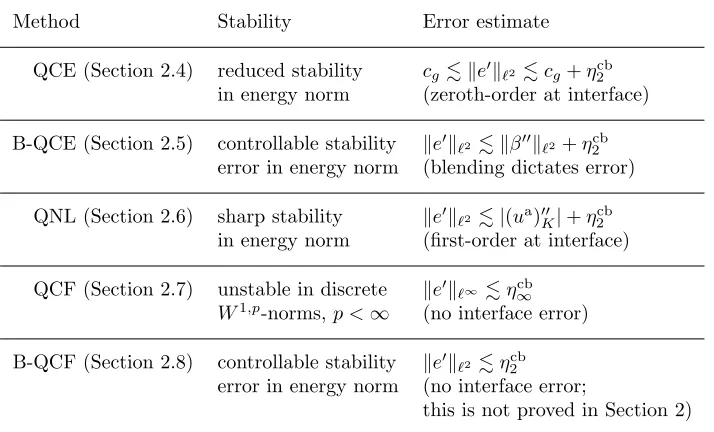
Table 2.1. Summary of stability results and error estimates formally derived in Section 2. Here,e:=ua−uac, andηcb_p :=(ua)p_{( ˜C)}+(ua)22p_{( ˜C)}.

Method Stability Error estimate

QCE (Section 2.4) reduced stability cge2 cg+ηcb₂

in energy norm (zeroth-order at interface)

B-QCE (Section 2.5) controllable stability e2β2+η₂cb

error in energy norm (blending dictates error)

QNL (Section 2.6) sharp stability e2|(ua)_K|+η₂cb

in energy norm (first-order at interface)

QCF (Section 2.7) unstable in discrete e∞ηcb_∞

W1,p_{-norms,p <∞ (no interface error)}

B-QCF (Section 2.8) controllable stability e2ηcb₂

error in energy norm (no interface error;

this is not proved in Section 2)

in Li, Luskin, Ortner and Shapeev (2013). Sharp stability results for the B-QCF method in a discreteH2-type norm are established by Lu and Ming (2013).

2.9. Summary of results

We briefly summarize the main results that we derived in this section in Table 2.1. To simplify the presentation, we introduce notation for the error e := ua −uac, and for the Cauchy–Born consistency error, η_pcb := (ua)p_{( ˜C)}+(ua)2₂p_{( ˜C)}, for a suitably defined (method-dependent)

con-tinuum region ˜C.

3. Atomistic simulation

In this section, we introduce an atomistic model for an infinite crystal. Some care must be taken with the formulation of the appropriate func-tion space setting, but it is well suited to discussion ofrates of convergence