Face Recognition at a Distance: a study of super resolution

(1)

M.Sc. Thesis

Yuxi Peng

University of Twente

Department of Electrical Engineering,

Mathematics & Computer Science (EEMCS) Signals & Systems Group (SAS)

P.O. Box 217 7500 AE Enschede The Netherlands

Report Number: SAS2011-014 Report Date: August 28, 2011

Period of Work: 01/02/2011 – 31/8/2011 Thesis Committee: Dr. ir. R.N.J. Veldhuis

(2)

Abstract

We evaluate the performance of face recognition using images with differ-ent resolution. The experimdiffer-ents are conducted on Face Recognition Grand Challenge version one (FRGC v1.0) database and Surveillance Cameras Face (SCface) Database. Three recognition methods are used, namely Principal Component Analysis (PCA), Linear Discriminant Analysis (LDA) and Local Binary Pattern (LBP). To improve the performance of face images with low-resolution (LR), two state-of-art super-low-resolution (SR) methods are applied. One is called Discriminative Super-resolution (DSR). It finds the relation-ship from low-resolution images to their corresponding high-resolution (HR) images so that the reconstructed super-resolution images would be close to the HR images which belongs to the same subject with them and far away from others. The other SR method uses Nonlinear Mappings on Coherent Features (NMCF). Canonical Correlation analysis is applied to compute the coherent features between the PCA features of HR and LR images. Then Radial Basis Functions (RBFs) is used to find the mapping from LR fea-tures to HR feafea-tures in the coherent feature space. The two SR methods are compared on both FRGC and SCface databases as well.

(3)

(4)

Acknowledgements

This thesis presents the work I have done in the Signals and Systems group in University of Twente. During the seven-month work, I have worked with a lot of people who contributed their time and efforts to my research. It is a pleasure for me to express my gratitude to them all.

First of all, I owe my deepest gratitude to Dr. ir. R.N.J. Veldhuis for supervision, advice, and guidance from the initial to the final level enabled me to develop an understanding of the project. His truly scientist intuition has made him as a constant oasis of ideas and passions in science, which exceptionally inspire and enrich my growth as a student wants to be. Special thanks are also given to Dr. ir. B. Gokberk for the advice, direct supervision and useful discussions throughout the project. I am also grateful to Dr. ir. L.J. Spreeuwers for giving me useful advice.

I gratefully thank Chanjuan Liu, who was always willing to offer help during my project. I would like to thank our technician Geert Jan Laanstra and our secretary Sandra Westhoff for administration support.

I would like to express my gratitude towards my parents and my friends for their encouragement and support during my study in the Netherlands.

(5)

(6)

List of Figures

1.1 Face recognition procedures. . . 1

3.1 Examples of eigenfaces. . . 14

4.1 Images from the first subject in ORL. . . 19

4.2 FRGC sample images. . . 20

4.3 SCface sample images. First row: distance1; second row: distance2; third row: distance3; last row: mug shot frontal images. . . 21

4.4 FRGC sample images with different resolution. First row: 64×64; second row: 32×32; third row: 16×16; fourth row: 12×12; last row: 6×6. . . 22

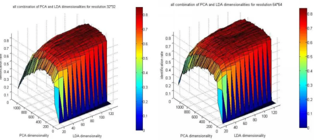
4.5 All combination of PCA and LDA dimensionalities. Left: 32×32; right: 64×64. . . 23

4.6 LDA results on three configurations. . . 24

4.7 Compare LBP with LDA . . . 24

4.8 LBP extra experiments. Left: with weight vs. without weight; right: all patterns vs. only uniform patterns. . . 25

4.9 SCface cropped images. First row: distance1; second row: distance2; third row: distance3; last row: mug shot frontal images. . . 27

4.10 Results of LDA tests of different PCA dimensionality. . . 28

4.11 FRGC sample images. First row: 56×48, second row: 42×36, third row: 14×12, last row: 7×6. . . 31

4.12 SCface cropped images, experiment 3. First row: distance1; second row: distance2; third row: distance3; last row: mug shot frontal images. . . 32

4.13 FRGC SR image construction using RL. . . 33

4.14 FRGC SR image construction using DSR. . . 34

4.15 DSR results on FRGC. PCA results. Left: input resolution 7×6; right: input resolution 14×12. . . 35

(9)

4.16 DSR results on FRGC. LBP results. Left: input resolution 7×6; right: input resolution 14×12. . . 36 4.17 DSR results on FRGC. LDA results. Left: input resolution

7×6; right: input resolution 14×12. . . 36 4.18 SCface SR image construction using FRGC for training. (1st

and 3rd row: distance1 LR images; 2nd and last row: corre-sponding SR images.) . . . 37 4.19 SCface SR image construction 2. 1st, 4th and 7th row:

dis-tance1 LR images; 2nd row: distance2 SR; 3rd row: distance2 HR images; 5th row: distance3 SR; 6th row: distance3 HR images; 8th row: distance2+3 SR. . . 38 4.20 Face recognition results of SCface using DSR . . . 39 4.21 ORL sample images. First row: 32×32 train; second row:

8×8 train; last row: 8×8 test. . . 39 4.22 NMCF results of different PCA dimensions on ORL. . . 40 4.23 NMCF results compared with [9]. . . 40 4.24 NMCF results of different PCA dimensions on FRGC. Left:

LR 7×6, HR 54×48; right: LR 14×12, HR 54×48. . . 41 4.25 Face recognition results of FRGC using NMCF. . . 41 4.26 NMCF results of different PCA dimensions on SCface. (a)

distance2 SR. . . 42 4.27 NMCF results of different PCA dimensions on SCface. (b)

distance3 SR. . . 42 4.28 NMCF results of different PCA dimensions on SCface. (c)

(10)

List of Tables

4.1 Information about selected cropped images . . . 27

4.2 Comparison of PCA[6], LDA and LBP. Identification rate[%]. 28 4.3 2nd configuration. Identification rate[%]. CAM1t stands for using images from cam1 for training. . . 29

4.4 3rd configuration . . . 30

4.5 Details of LBP and LDA parameters. . . 35

4.6 DSR results on SCface . . . 38

4.7 Number of PCA vectors chosen for FRGC . . . 41

4.8 NMCF results on SCface . . . 43

(11)

(12)

1 Introduction

1.1 An introduction to face recognition

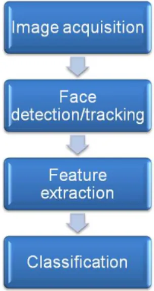
Face recognition has become an attractive research field in recent decades. Given a face image, face recognition system automatically identify or verify a certain individual [26]. Usually, face recognition follows the procedure in Figure 1.1.

Figure 1.1: Face recognition procedures.

Image acquisition: the first stage is to obtain images containing facial re-gion. Different acquisition devices are used for different situation. The most popular device for capturing two-dimensional (2D) images is the charge-coupled device (CCD) camera. Three-dimensional (3D) images are usually acquired by stereo of the images captured by two cameras placed on the left and right. Infrared camera is also used in some situation such as night time. Face detection/tracking: when images are available, we need to locate

(13)

the faces in them. In videos, faces may have to be tracked for a certain time to obtain better quality images.

Feature extraction: at this stage, useful data is extracted for recognition. Some pre-processing approaches might be needed before extracting features, for instance, using image segmentation method to crop the face region. The images may need alignment and normalization as well. Then the global or local features will be extracted from the face images.

Classification: when the image features are extracted, they are fed into a classifier for identification or verification. The system will declare a decision about the identity of the subject.

Face recognition systems can obtain promising results when using high-resolution (HR) frontal images, but face recognition at a distance (FRAD) is still challenging. The face regions of images acquired at a distance are usually small and has low quality. Face recognition task can be more difficult in surveillance situation.

To deal with the low-resolution (LR) problem of images acquired from long distance, super-resolution (SR) methods can be applied. Super-resolution methods try to enhance the Super-resolution of an image. In this report, face recognition performance of low-resolution images is evaluated and two state-of-art super-resolution methods are compared.

1.2 Purpose of our research

The objective of our research is to find out the influence of low-resolution images to face recognition system and how the state-of-art super-resolution approaches would improve the recognition performance.

1.3 Outline of the report

The content of this report is arranged as follows:

Chapter 2: literature review. In this chapter, we review previous work on face recognition at a distance and super resolution.

Chapter 3: algorithms. Three important face recognition methods and two state-of-art super-resolution algorithms are introduced.

Chapter 4: experiments. This chapter includes database description and all the experiments we have conducted. For each experiment, the experi-ment configuration is first introduced, then the experiexperi-mental results and the discussions are presented.

(14)

2 Literature review

In this chapter, firstly the main problems of face recognition at a distance are described and several recent studies on face recognition at a distance are introduced. Then super-resolution methods for both visual enhancement and face recognition are discussed.

2.1 Face recognition at a distance

Although face recognition algorithms obtain high recognition rates in close proximity, great challenge still exists in long distance which is also referred to as face recognition at a distance. Why face recognition at a distance different? First, it’s hard to ensure the quality of images. Second, long-distance face recognition is usually used for surveillance without cooperation of users. In addition, it may need to work 24 hours and in outdoor condition. Issues like lighting and weather condition are significant problems. It may also deal with multi-faces.

Problems of FRAD

The main problems and some relevant solutions of FRAD are stated in Chap-ter 6 of [19]. Firstly, the images captured at a distance are usually with low resolution which will lead to low recognition accuracy. Using high-definition camera is a possible solution but it can result in decreasing of speed of de-tection. Secondly, interlace is a problem in video images. It happens when the faces are moving fast enough that each video frame is captured at a different position. A progressive scan video system can reduce the chance of interlace. Thirdly, in many cases of FRAD the face is blurred because it is out of focus of the lens. The degree of blur can be decreased by small aper-ture lens. Fourthly, motion blur also happens frequently in FRAD when the face is moving fast or the camera is shaking. Rapid exposures can be used to avoid this problem, but the aperture stop would be increased which

(15)

flicts to the out-of-focus problem. Furthermore, in FRAD especially under surveillance situation, it is also important to cover most users’ heights and capture frontal faces. Besides, weather and atmospherics, such as thermal waves, have a significant impact on recognition accuracy [19].

A FRAD system for pose variation

In [14], some solutions to different aspects of face recognition at a distance especially for pose variation problem are proposed. To obtain good quality images, two different cameras are used. A wild field camera is placed in a fixed position and a foveal camera is placed on a pan/tilt platform. The output of the wild-field camera is used to orient the foveal camera at faces.

They developed a robust face detection approach combining three modal-ities: 2-frame motion differencing, background subtraction and skin color detection. These three modalities can make up for the weakness of each other. For each pixel in an image, the possibility of it being a face pixel is modeled as a mixture of Gaussian distributions of the results of the three modalities. In order to track an individual, a fixation prior is introduced which causes the camera to dwell on the person. When a face is successfully detected, a feedback map is generated to inhibit this position temporarily so that the system would move to a different position for next detection.

In the pre-processing phase, a cascade-based face detector is employed. Firstly, twenty landmarks on the face is found by combining a local likelihood model learnt from a training dataset and a Gaussian model of the covariance of the twenty feature points. Then a warp is performed by triangulating the images based on the landmarks and mapping the vertices of the triangle to the standard shape. Finally, the features are extracted by placing a regular grid of 25 squares centered on each landmark and computing the average gradient in eight directions and the mean intensity level. These extracted features are correlated across different poses.

A one-to-many mapping from an identity space without pose varia-tion to the observed data space is proposed to deal with various poses for recognition. This mapping is learnt from a training set using expectation-maximization (EM) algorithm. For input images, the mapping can be ap-plied to obtain the corresponding features in the identity space. Thus, a simple way to perform recognition is to use nearest neighbor classifier on these features.

(16)

2.1 Face recognition at a distance 5

3D model for pose problem in FRAD

In [11], a prototype system to locate, track and identify people going through a predefined zone is proposed. The system focus on detection and tracking and pre-processing. A single ultra-high resolution camera is used to capture images. This system locates a human head by locating the entire body of a person. Moving subjects are detected using background subtraction while static subjects are detected using model-based detection module which employs Edgelet features. Elliptic shape mask and an appearance map are applied when tracking subjects under difficult crowd conditions.

Because this long-distance face recognition is without user cooperation, frontal images are not always obtained. 3D models are used to deal with pose problem. The pose of the acquired images is initially estimated us-ing a tracker which combines a recursive and key-frame based approach to minimize tracking drift and jitter. Then a two-stage 3D-reconstruction is applied. First, optimal poses are selected and corresponding points are back-projected and intersected to determine the 3D position. Second, the individual reconstructions are integrated into a single 3D point cloud. A mesh description of the dense cloud of points is inferred based on the ap-proximation of the head geometry.

The reconstructed 3D models are nice for both indoor and outdoor sit-uations. However, the 3D recognition has not been tested.

Magnifications and recognition rate

A database acquired from long distances and with high magnifications and proposed an algorithm to deal with magnification blur is presented in [25]. Indoor images and video sequences are taken at distance 10 to 16 meters by a commercially available pan tilt zoom (PTZ) camera. The images are cap-tured ar different distances. System magnification and illumination changes are present in the images. The gallery images are taken at 0.5 m distance. The outdoor images and video sequences are captured by a Meade ETX-90 telescope coupled with a JVC MG-37U camcorder. The subjects have two motions: standing still and walking. The gallery images are taken at 1 m at indoor situation.

(17)

coefficients are applied. Adaptive grey level contrast stretching is applied then and output image is reconstructed by the corresponding inverse wavelet transform. Lasso regularization is used for recognition. This wavelet based algorithm increases recognition rate. But as magnification increases, im-provement decreases.

Close, medium and far distance scenarios

Close, medium and far distance face recognition in segmented faces are an-alyzed in [13]. Two recognition system is used. One uses Principal Compo-nent Analysis (PCA) with Support Vector Machine (SVM) classifier. The other one applies Discrete Cosine Transform (DCT) with Gaussian Mixture Model (GMM) classifier. The images are manually marked with “close” , “medium” and “far” distance based on whether the image contains only head and should or the upper body or the full body. The faces are seg-mented using the VeriLook SDK and the errors are corrected by manually marking the eyes. The quality assessment shows that, for full images, the farther the distance the higher the entropy while the opposite occurs for segmented images. Then the recognition performance of PCA-SVM system and DCT-GMM system are evaluated. Half of the close distance images are used for training. The other half of close distance images as well as medium and far distance images are used for testing. The results indicate that the recognition accuracy decreases as the distance increases. And GMM-based system works better in far distance conditions.

This work is extended in [20] by the same authors. They make the fusion of the previous two face verification methods to obtain better results. A “distance index” is defined to estimate distance:

D=−log(As/Af)

where As stands for segmented face area and Af is full image area. Two

ways of fusing the recognition methods PCA-SVM and DCT-GMM are as follows:

Fixed fusion: s= (sDG+sP S)/2;

Adaptive fusion: s= (D/2)sDG+ (1−D/2)sP S

wheresDG andsP S are the scores obtained by PCA-SVM and DCT-GMM

respectively, andsis the score of fusion.

(18)

2.1 Face recognition at a distance 7

A surveillance system

In [23], a complete system for surveillance is proposed. The image acquisi-tion setup is a co-located pair of Wide Field Of View (WFOV) and Narrow Field Of View (NFOV) cameras with a high-end but standard workstation containing Matrox frame grabbers to accept the video streams. The aim of the systems is to detect and track people moving in the field of view of the fixed WFOV camera, so background subtraction is used for detection. And the NFOV camera view is calibrated with respect to the WFOV camera view. WFOV camera detects multiple subjects and uses a priority mecha-nism to select a target for NFOV camera. Every target has a score in his target record. The score is determined by the distance, direction, speed, etc. The subject that is more likely to leave the region will be selected first. Once a subject is selected, the filter will predict the location of his/her face at about 0.5 to 1.0 sec. The NFOV camera will zoom in and wait for the target to show up. And the resolution will increase by 20% each time the same target’s image is captured.

The faces are detected by Pittsburgh Pattern Recognition FT-SDK and cropped for next procedure. Face recognition is operated asynchronously. And the result will be passed to the target scheduler to update target record. Several commercial recognition methods are available in this system. In the detection experiment, they report one failed person detection and eight failed face captures out of 466 trials, usually due to the subject or face being obscured in some manner. The recognition result of Cognitec FaceVACS shows all successful recognition and most are recognized at 16 to 20 meters.

Stereo reconstruction for FRAD

(19)

The authors extended their work in [15]. A combination of Viola-Jones detector and skin detector is used to identify possible facial regions and find the landmarks. To reconstruct 3D features, a dense, global stereo matching is first performed using global optimization algorithms. Then AAM is used to find sparse correspondences of the left and right images of the stereo pair. The experimental results have slightly improvement comparing to their work in [16]. However, these methods can not deal with expression variations. In their later research, texture is also used to obtain better results [17][18].

2.2 Super resolution

In the field of face recognition at a distance, most of the previous works focus on better image acquisition systems such as using high-quality cameras to improve the quality of captured images. However, when low-quality images are obtained, an intuitive approach of improving the quality of images is super-resolution. Super-resolution was designed at first to construct high-resolution images for visual enhancement. Some of the SR methods attempt to accumulate information of several low-quality images to reconstruct one super-resolved image. Since enough images would not always be available, researchers focus on reconstructing high-resolution image from only one LR input in recent years.

2.2.1 SR for visual enhancement

Three SR methods are proposed in Chapter 7 of [4]. The first one is called closed-loop super-resolution. It uses Generic 3D face model to improve the resolution of 3D texture. Bilinear basis images are obtained for further esti-mation of the pose and illumination coefficients. The SR method proposed in this paper is extended from an iterative back-projection (IBP) method to 3D. The SR texture is constructed separately based on six facial regions: eyes, eye brows, mouth and other parts to handle expression changes. And the super-resolution 3D facial texture is fed back to generate low-resolution bilinear basis images. Because the method has feedback mechanism, the quality of SR images becomes better as the number of frames used grows. This method can deal with illumination and expression, but the images are almost frontal images and their expression can’t change too much.

(20)

2.2 Super resolution 9

parts. A match statistics is designed to measure the alignment. The SR results demonstrated that the proposed deformation method is much better than global registration.

The third one deals with side view face images in video. A face image is acquired by cutting the upper 16% of the segmented human body. Elastic registration method is used for motion estimation and a match statistic is introduced to detect and discard images that are poorly aligned. Then an iterative method is proposed to construct high-resolution images. In this approach, multiple low-resolution images are needed to reconstruct a high-resolution image.

2.2.2 SR for recognition

Though the super-resolution methods focus on visual enhancement have achieved great success, the objective of most SR methods is to construct high frequency details which is not sufficient for recognition of low-resolution images. Recently, some methods were developed for face recognition per-spective. Here we briefly explain some of them.

S2R2

In [7], an algorithm called simultaneous super-resolution and recognition (S2R2) is proposed. A high-resolution training set is needed and let F be the super-resolution feature which is provided by the training set. For an input low-resolution probe image Ip and the class kis claimed, first task is

to solve the problem

Xp= arg min x

kBx−Ipk2+α2kLxk2+β2kF x−F Igk2 (2.1)

whereIg is the gallery image with classk. Matrix B is the linear model for

downsampling the HR image x to its corresponding LR imageIp. Lx is a

vector of edge values in whichLis first or second derivative approximation.

αis a regularization parameter. βis an additional regularization parameter. Then the distance is measured by a combination of the residual norm on each set of model assumptions in Equation (2.1).

(21)

MDS

In [5], a novel approach for improving the matching performance of LR images using multidimensional scaling (MDS) is proposed. Their goal is to find a transformation matrix that the distance between transformed features of LR images can be as close as possible to their corresponding HR images. LetIh andIl represent for HR and LR images, andW is the transformation matrix. The objective function is described as following

J(W) = λ

N X i=1 N X j=1 ( W

T₍_φ₍_Il

i)−φ(Ijl))

−

φ(I

h

i)−φ(Ijh)

)

2

+(1−λ)

N X i=1 N X j=1

δ(ωi, ωj)

W

T₍_φ₍_Il

i)−φ(Ijl))

2

(2.2)

whereφ(x) can be a linear or non-linear function of the input feature vec-tors. λ controls the relative effect of the distance preserving and the class separability on the total optimization. A simple way of make use of class in-formation is thatδ(ωi, ωj) is set to one whenIiandIjare from the same class

and otherwise it is set to zero. This specific form makes sure the distance between data from the same class to be small. The iterative majorization algorithm is used to minimize the objective function.

In testing phase, for input imageIinput, the transformed feature ˆIinput is

obtained by

ˆ

Iinput=WTφ(Iinput) (2.3)

Euclidean distance is then computed for classification.

Their experimental evaluation shows that this method performs better than bicubic interpolation and a super-resolution method using sparse rep-resentation [24].

CLPM

In [10], a SR method using coupled locality preserving mappings (CLPM) is proposed. This method requires HR and LR image pairs for training. The main idea is to obtain coupled mappings which can project both HR and LR image features to a unified feature space so that direct comparison of HR and LR in that feature space could be possible.

The objective is to make sure the projections of LR images and their corresponding HR images would be as close as possible in the new unified feature space. Let Ih and Il be the HR and LR images, this can be formu-lated as

J(fL, fH) = N X i=1 P T

LIil−PHTIih

2

(22)

where PL and PH are the transformation matrix from LR and HR image

space to the unified feature space. We can obtain the mappings by min-imizing this formula. The gallery and probe images then will be mapped to a unified feature space where we can use nearest neighbor classifier for recognition.

This method has good performance on face recognition. Besides, it is more suitable for real-time systems because the test process can be very fast once the training part is done offline.

Key-frames for long video sequences

A face recognition system for long video sequences is presented in [12]. It selects key-frames and then applies hybrid super-resolution. Key-frames are chosen as follows. First, the most frontal images are selected using auto-associative memories. Then, a quality score is assigned to each frontal image by a face quality assessment (FQA) and the images with higher score are kept for next procedure. Lastly the selected images are aligned with the best one. The next step is hybrid super-resolution. Multiple images from the key-frames are used to construct a HR image. Multi layer perceptron (MLP) is applied then to further improve the constructed HR image. Finally, a face recognition algorithm that is sensitive to degradation in its input is used for testing the performance. This system has better results than Schultz[12] and Baker[15] and can be a good way to improve the recognition rate when long video sequences are available. Nonetheless, the performance of this system on images with lower solution is unknown since the LR images used in this paper are 46×56 pixels.

DSR and NMCF

(23)

(24)

3 Algorithm introduction

3.1 Face recognition methods

3.1.1 Eigenface

Principal Component Analysis (PCA), or the eigenface method, is a widely used basic face recognition algorithm [21]. It provides a simple approach to extract the information contained in a face image to capture the variation of a collection of face images, and the information is used to encode and compare individual images.

Given a training set ofN images ({I}={Ii}Ni=1), first compute the mean image ¯I = _N1 PN

i=1Ii. Then substract the mean from each face ˆIi =Ii−I¯.

The convariance matrix is computed as following

C = 1

N

X

i=1 ˆ

IIˆT =AAT (3.1)

where the matrix A={Iˆi}Ni=1. Then solve the eigenvalue problem

Λ =VTCV (3.2)

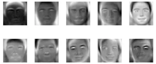
whereV is the eigenvector matrix ofCand Λ is the diagonal matrix contain-ing eigenvalues ofC on its main diagonal. The eigenvectors are then sorted so that their correponding eigenvalues are in descending order. These vec-tors are called eigenfaces, see Figure 3.1. Usually, the number of pixels in the images (M) would be relatively larger than the number of images in the training set (N). Thus, the complexity of calculation is reduced.

In testing phase, an input image Iinput is transformed to its eigenface

featureXinput by

Xinput=VT(Iinput−I¯). (3.3)

Then eigenface features Xi and Xj are compared using Euclidean distance

or cosine distance. Three methods for distance measure is introduced in

(25)

Figure 3.1: Examples of eigenfaces.

pendix. The one that gives best results is used in the experiments discussed in Chapter 4.

3.1.2 Fisherface

Fisher’s Linear Discriminant (FLD) method, or Linear Discriminant Anal-ysis (LDA) selects projection vectors in such a way that the ratio of the between-class scatter and within-class scatter is maximized [3].

Given a training set of N images ({I} ={Ii}Ni=1), assume they belong to m different classes {Ci}m_i₌₁ that each class has Ni images. Define the

between-class scatter as

SB = m

X

i=1

Ni(µi−µ)(µi−µ)T

and the within-class scatter as

SW = m

X

i=1

X

Ik∈Ck

(Ik−µi)(Ik−µi)T

whereµ is the mean image of training set, and µi is the mean ofith class.

Then the optimal projection is selected to maximize the ratio of the between-class scatter and within-between-class scatter as following

Wopt= arg max W

WTSBW

|WT_S WW|

(3.4)

whereW can be solved as the eigenvectors of

SBW = ΛSWW. (3.5)

However,SW is always singular because the rank ofSW is at mostN−m

(26)

3.1 Face recognition methods 15

then apply the standard FLD as discussed above to reduce the dimension tom−1. Thus, the projection is computed as follows

Wopt=WpcaT Wf ldT .

In testing phase, an input imageIinput is projected to Fisherface feature

space by

Xinput=Wopt(Iinput−µ). (3.6)

Different methods of distance measure can be used to compare the features while cosine distance which has the best performance is used in our experi-ments.

Because the Fisherface method is the only LDA method used in our experiments, we will call it LDA for the rest of this report.

3.1.3 LBP

Local Binary Pattern (LBP) operator was originally designed for texture description [1]. For a 3×3 neighborhood, LBP assigns a label to each pixel except the center one according to their values and the value of the center pixel. More specifically, if the value of one pixel is smaller than the value of the center pixel, it’s label is assigned to 0; otherwise, it is assigned to 1. Thus, an 8 bit binary value is generated for this neighborhood. Then the histogram of the labels can be used as a texture descriptor. This 3×3 neighborhood is also refered as (8,1) neighborhood which means eight sampling points on a circle of radius of one. Besides, (8,2) and (16,2) neighborhoods are also commonly used.

A local binary pattern is called uniform if it contains at most two bit-wise transitions from 0 to 1 or 1 to 0 when the bit pattern is considered circular. For example, 11111111 (0 transitions), 00000011 (2 transitions) and 11100001 (2 transitions) are uniform patterns while 11001001 (4 transi-tions) and 01100101 (6 transitransi-tions) are not. Using only uniform patterns for LBP means that each uniform pattern has a seperate bin and all nonuniform patterns are assigned to one bin when computing the histogram. It has been demonstrated in [1] that uniform patterns account for 90 percent of all pat-terns in the (8,1) neighborhood using images from the Facial Recognition Technology (FERET) database.

In face recognition process, the basic histogram can be extended to a spatially enhanced histogram. Each image is divided to several facial regions and the LBP histogram is computed for each region. Then the histograms are concatenated to build a global description of a face.

The common method for distance measure of LBP is the weighted Chi square distance which is defined as

χ2_w(x, y) =X

j,i

wj

(xi,j−yi,j)2

xi,j+yi,j

(27)

whereirefers toith bin in histogram corresponding to thejth region of the image, andwj is the weight of regionj.

3.2 Super resolution methods

Two state-of-art super-resolution methods are used in our experiments.

3.2.1 RL and DSR

A super-resolution method for very low resolution is proposed in [27]. Very low resolution (VLR) face recognition problem is defined as the situation that face region is smaller than 16×16 pixels in this paper. A new data con-straint is proposed for relationship learning based super-resolution. Given a set of HR and VLR image pairs ({I_ih, I_il}N

i=1 ), let R be the relationship between HR and VLR space. The idea is to minimize the distance between HR and the space of VLR projected by R, see Equation (3.8).

R= arg min

R0 N X i=1 I h i −R0Iil

2

(3.8)

Then a SR image can be constructed from a given LR image Iinput by

ISR =RIinput. This method is called RL, which is used for reconstructing

high-resolution images.

Furthermore, discriminative super-resolution (DSR) is proposed to ac-quire better results in face recognition. This method makes use of class information of the training data to make sure the reconstructed HR images are clustered with the images from the same class and far away from those from other classes. A distance function (Equation (3.9)) is introduced to the minimization problem.

d(R) = mean(

I

h i −R0Ijl

2

|class(I_ih) = class(I_jl))

−mean(

I

h i −R

0_Il j

2

|class(I_ih)6= class(I_jl)) (3.9)

Then the DSR formula integrates Equation (3.8) and (3.9)

˙

R= arg min

R0 1 N N X i=1 I h i −R

0_Il i

2

+γd(R0) (3.10)

whereγ is a constant to balance the above two terms. In our experiments,

γ is set to 1.

Thus, for a given image Iinput, we first applyISR0 = ˙RI_input, and then

(28)

3.2 Super resolution methods 17

3.2.2 NMCF

The super-resolution approach using nonlinear mappings on coherent fea-tures (NMCF) is proposed by Huang et al. in [9]. First, PCA feafea-tures are extracted to reduce computational costs. Given a training set of HR and LR image pairs ({IH, IL}={I_ih, I_il}N

i=1), PCA features of them are defined asXH ={xh_i}N

i=1 and XL={xli}Ni=1 and extracted by

xh_i = (VH)T(I_ih−I¯H), xl_i = (VL)T(I_il−I¯L) (3.11)

whereVH andVL are the corresponding eigenvectors of the covariance ma-trices (IH −I¯H)(IH −I¯H)T and (IL−I¯L)(IL−I¯L)T, and ¯IH and ¯IL are the mean of the HR and LR images respectively. Then Canonical Cor-relation Analysis (CCA) is used to project PCA features to a new coher-ent feature space. First we subtract the mean ¯X from the PCA features:

ˆ

XH ₌_XH ₋_X¯H_{, ˆ}_XL₌_XL₋_X¯L_{. Let} _WH _and _WL _{be the base vectors,}

the coherent features of HR and LR are

CH = (WH)TXˆH, CL= (WL)TXˆL. (3.12)

To maximize the correlation between HR and LR coherent featuresCH and

CL, the correlation coefficient is defined as

ρ = E[C

H_CL_]

p

E[(CH₎2_]_E_[(_CL₎2_]

= E[(W

H₎T_XˆH_{( ˆ}_XL₎T_WL_]

q

E[(WH₎T_XˆH_{( ˆ}_XH₎T_WH_]_E_[(_WL₎T_XˆL_{( ˆ}_XL₎T_WL_]

(3.13)

whereE[·] stands for mathematical expectation. DefineC11=E[ ˆXH( ˆXH)T] and C22 = E[ ˆXL( ˆXL)T] as the within-set covariance matrices and C12 =

E[ ˆXH( ˆXL)T] andC21=E[ ˆXL( ˆXH)T] as the between-set covariance matri-ces. Compute

R1=C11−1C12C22−1C21, R2 =C22−1C21C11−1C12. (3.14)

Then the base vector WH is made of eigenvectors of R1 and WL is made of eigenvectors of R2 when their corresponding eigenvalues are sorted in descending order. The last step of training is to use Radial Basis Functions (RBFs) to learn the relationship between the coherent features of HR and LR. RBFs are used to build up function approximations of the form

f =

N

X

j=1

(29)

where the approximating function f is represented as a sum of N radial basis functions, each associated with a different center tj with weighting

coefficientωj. Multiquadric basis function

ϕ(kt−tjk) =

q

kt−tjk2+ 1

is chosen for the implementation. The goal is to build the mapping between HR and LR coherent features CH and CL. Thus, by setting f = ch_i and

t=cl_i, Equation (3.15) is represented as CH =WΦ, specifically

[ch₁, . . . , ch_n] = [ω1, . . . , ωn]





ϕ(cl₁−cl₁). . . ϕ(

cl_n−cl₁) . . . .

ϕ(cl₁−cl_n). . . ϕ(

cl_n−cl_n) 

. (3.16)

So the weight matrix W can be solved by

W =CH(Φ +τ Iid)−1 (3.17)

whereτ Iid is added because Φ is not always invertible. τ is a small positive

value such as 10−3, and Iid is identity matrix.

In testing stage, for HR gallery images IG ={I_ig}M

i=1, coherent features are computed as following

xg_i = (VH)T(I_ig−I¯H),

cg_i = (WH)T(xg_i −X¯H).

For a LR probe imageIp _{first we compute the coherent feature}

xp = (VL)T(Ip−I¯L),

cp= (WL)T(xp−X¯L).

Then apply the learnt mapping to obtain the corresponding SR features by

cSR=W ·[ϕ(

c

l

1−cp

). . . ϕ(

c

l N −cp

)]

T_. _(3.18)

Then the above features are feed to the nearest neighbor classifier for recog-nition

classify(cSR) = min(kcSR−cgik

(30)

4 Experiments

In this chapter, first the databases used in our experiments are introduced. Then we show the face recognition results of images with different resolution and evaluate the performance of two state-of-art super-resolution methods. In all the experiments, image identification is performed other than verifica-tion. That is, for an input probe image, the distances between it and each gallery images are computed in the recognition phase and it is assumed to have the same class as the image which has the smallest distance with it.

4.1 Database description

4.1.1 ORL

Olivetti Research Laboratory (ORL) database contains ten images of each of 40 distinct subjects. The images have slightly various poses, expressions and illumination conditions. The size of each image is 92×112 pixels. The ten images from the first subject is shown in Figure 4.1.

Figure 4.1: Images from the first subject in ORL.

(31)

4.1.2 FRGC v1.0

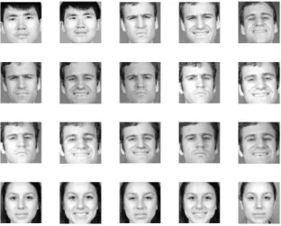
Face Recognition Grand Challenge version one (FRGC v1.0) database con-tains controlled images which were taken in a studio setting and uncontrolled images which were taken in varying illumination conditions. In our exper-iment, only 2820 controlled high-quality images are used. These images are all frontal images with two expressions (smiling and neutral). The im-ages in Figure 4.2 are cropped according to the upper-left and lower-right coordinates provided in the database and turned into gray-scale.

Figure 4.2: FRGC sample images.

4.1.3 SCface

Surveillance Cameras Face (SCface) Database contains 4,160 static images of 130 subjects. They have five surveillance cameras namely cam1, cam2, cam3, cam4 and cam5. Cam1 and cam5 were also used for infrared (IR) night vision mode which named cam6 and cam7. These cameras each took one photos of each subject at three distances, 4.20 meters (distance1), 2.60 meters (distance2), and 1.00 meter (distance3). IR mug shots were taken by cam8. Another set of images were taken by a mug shot camera at day time. Nine images per subject provide nine discrete ranging from left to right profile in equal steps of 22.5 degrees including a mug shot frontal image at 0 degree [6]. Sample images from SCface are in Figure 4.3. Note that although images from distance3 are with higher resolution than distance1 and distance2, the pose variation is much more serious.

(32)

4.2 The influence of different image resolution 21

Figure 4.3: SCface sample images. First row: distance1; second row: dis-tance2; third row: distance3; last row: mug shot frontal images.

to 64×64 and masked with an elliptical mask. 501 images were randomly chosen as training images from the FERET database, one image per person. The frontal images taken by mug-shot camera in the SCface were put into th gallery set. For experiments at night, cam8 was also used as gallery. Images from each camera were used as probe each time. The performance of base-line PCA was evaluated using 40% eigenvectors, which is a 200 dimensional subspace. The rank-1 recognition rate varies from 1% to about 8%.

In our experiments, the mug-shot frontal images and the images from cam1 to cam5 taken at day time are used.

4.2 The influence of different image resolution

This experiment evaluates the influence of images with different resolution on FRGC v1.0 database.

4.2.1 Configuration

(33)

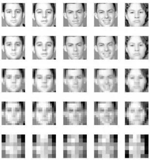
64×64, and 96×96, see figure 4.4.

Figure 4.4: FRGC sample images with different resolution. First row: 64×

64; second row: 32×32; third row: 16×16; fourth row: 12×12; last row: 6×6.

The 2820 images were divided into training, gallery and probe sets in different ways to find the best configuration:

1st: training set contains images from the first 80 persons and all images from the persons who have less than four images (including four). This training set contains 1228 images of 139 persons. Two images per person from the rest images are used as gallery images (242 images) and the others as probe images (1350 images).

2nd: training set contains 812 images of 109 persons from 1st training set. Gallery and probe sets are the same as the 1st configuration.

3rd: training set contains 400 images of 76 persons from 1st training set. Gallery and probe sets are the same as the 1st configuration.

(34)

4.2 The influence of different image resolution 23

So 3×3 windows cannot be used for images with resolution lower than 9×9. And 4×4, 5×5, 6×6, and 7×7 windows cannot be used for images with resolution lower than 12×12, 15×15, 18×18, and 21×21 respectively. The weight of each window was assigned based on the recognition rate of performing LBP on training sets using only one window each time.

4.2.2 Experimental results

LDA

Proper number of eigenvectors for both PCA and LDA part must be chosen to obtain better results of LDA method. All combination of PCA and LDA dimensionalities were tried on resolution 32×32 and 64×64 for 1st configu-ration (see Figure 4.5). The recognition accuracy reach a maximum number 85.11% when PCA/LDA feature dimensionalities are 350/120 or 430/130 for resolution 32×32. And the highest rate of 64×64 is 84% when PCA dimensionality is 350 and LDA dimensionality is 130.

Figure 4.5: All combination of PCA and LDA dimensionalities. Left: 32×32; right: 64×64.

According to the results shown above, the number of PCA vectors were chosen as the minimum of 350 and the image dimensionality and the the number of LDA vectors were chosen as the minimum of the number of classes minus one and the image dimensionality for the next experiment. Then we applied LDA on the three different dataset configurations.

(35)

Figure 4.6: LDA results on three configurations.

LBP

Then we performed LBP using different number of windows and compared the results with LDA method on 1st configuration which gives the best results according to the previous experiment, see Figure 4.7.

Figure 4.7: Compare LBP with LDA

(36)

4.3 Surveillance camera results 25

LDA especially when more windows are divided because the local binary features must be computed for each window and for each image.

Two more experiments were performed using LBP to find out the influ-ence of weight in distance measure and the differinflu-ence between using uniform patterns and using all patterns (Figure 4.8). The Chi square distance with weight has 1% to 3% better results than these without weight. And using all patterns instead of only uniform patterns slightly improves the results (except for 7×7), but it reults in much longer computation time.

Figure 4.8: LBP extra experiments. Left: with weight vs. without weight; right: all patterns vs. only uniform patterns.

4.2.3 Discussion

In general, as the resolution become lower, the recognition rate decreases. LDA performance decreases slightly but still remains the same level when image resolution is higher than 16×16 and LBP performance becomes stable when image resolution is higher than 32×32. A sharp decrease happening when images are smaller than 12×12 pixels indicates that some important information for LDA recognition is missing when a image is less than 12×12 pixels.

4.3 Surveillance camera results

(37)

4.3.1 Configuration

The images of surveillance from came1 to cam5 and the frontal images of mug-shot camera from SCface database were used. There are 130 subjects in SCface database. The mug-shot camera took one frontal image of each subjects. And the five surveillance cameras took one image per person per distance. So we have 650 images for each distance and 130 mug-shot frontal images. 2820 high-quality cropped images of 260 persons from FRGC v1.0 database were also used.

We have three dataset configurations in this section as well described as follows.

1st: 2820 high-quality images from FRGC are used as training images. Gallery images are the frontal images from SCface database and the images taken by camera 1 to 5 are probe images.

2nd: only images from SCface database are used for this configuration. Images taken by one camera are used as probe images at a time; images from the other four cameras are used as training set both separately and all together for each distance. Gallery images are the mug shot frontal images. 3rd: only images from SCface database are used for this configuration. Images are divided into four datasets: distance1, distance2, distance3 and mug shot frontal images. The first three sets are used for training and testing in turn. And the fourth set is gallery.

Two face recognition methods LDA and LBP were used. Cosine angle was used to measure distance for LDA the same as in the previous section. As demonstrated in Figure 4.8, the Chi square distance provides similar results with weight or without weight. Thus, Chi square (or weighted Chi square with weights set to one) was used for LBP in the following experi-ments. The other parameters of LBP were the same as in Section 4.2.

Face cropping

(38)

distance between eyes image size left eye coordinates

distance1 12 pixels 27×31 [7,7] distance2 22 pixels 45×45 [11,10] distance3 36 pixels 81×82 [21,17]

Table 4.1: Information about selected cropped images

Figure 4.9: SCface cropped images. First row: distance1; second row: dis-tance2; third row: distance3; last row: mug shot frontal images.

FRGC as training set

The proper number of PCA/LDA vectors still needs to be found for LDA method. We only tested the influence of PCA vectors because using maxi-mum number of LDA vectors can be good enough according to the results of previous experiments. The FRGC images are used for training, and mug-shot frontal images are used as gallery. The images from each distance are probe images.

We can see from Figure 4.10 (a) that the identification rate of distance3 reaches the highest number of 8.15% when PCA dimensionality is 50 and then keeps dropping after 200. This trend is quite similar to both distance2 and distance1. So only the results between 10 and 150 for these two distances are shown in Figure 4.10 (b) and (c). Then we chose to use PCA/LDA pair 50/50 for the following experiments.

(39)

(a) distance3

(b) distance2 (c) distance1

Figure 4.10: Results of LDA tests of different PCA dimensionality.

distance1 distance2 distance3

PCA LDA LBP PCA LDA LBP PCA LDA LBP

CAM1 2.3 10.0 7.0 7.7 12.3 27.0 5.4 9.2 17.7 CAM2 3.1 7.0 11.5 7.7 13.1 17.7 3.9 7.7 15.4 CAM3 1.5 6.2 8.5 3.9 7.7 16.2 7.7 7.0 13.9 CAM4 0.7 10.8 5.4 3.9 16.2 17.7 8.5 9.2 20.0 CAM5 1.5 6.2 9.2 7.7 10.0 13.1 5.4 7.7 13.8

Table 4.2: Comparison of PCA[6], LDA and LBP. Identification rate[%].

(40)

training set was used in this section. The performance of LDA and LBP is better than PCA, but the conclusion is similar: the distance influence the results, but results from distance3 are not as good as distance2. This is because images taken at distance3 are more of the top part of the head which can be seen in Figure 4.9. Furthermore, LBP outperforms LDA at distance2 and distance3.

2nd configuration

The experiments discussed above were using FRGC as training set. The performance was also evaluated when images from SCface are used as train-ing images as discribed in the 2nd configuration. For example, if cam5 is used as testing set, the training sets are cam1, cam2, cam3, cam4, and all images from cam1 to cam4. Both training and testing images are from the same distance, except gallery images are always the mug-shot frontal images. This experiment is only applied on LDA because the difference between the two configurations is the training set used and LBP does not need a training set.

CAM1t CAM2t CAM3t CAM4t CAM5t Allt

dist1

CAM1 – 10.00 10.00 7.69 7.69 19.23 CAM2 3.08 – 2.31 3.85 3.85 22.31 CAM3 4.62 4.62 – 3.85 4.62 18.46 CAM4 10.00 8.46 7.69 – 9.23 16.15 CAM5 7.69 7.69 6.92 9.23 – 14.62

dist2

dist3

Table 4.3: 2nd configuration. Identification rate[%]. CAM1t stands for using images from cam1 for training.

(41)

lot. Besides, comparing Table 4.3 with Table 4.2, using images from SCface as training set gives much better results than using FRGC.

3rd configuration

In [27], 10 images (5 LR images and 5 HR images) per subject from SCface are used and the results of eigenface, kernal PCA and SVM are all around 15% without super-resolution and 20% with the proposed super-resolution method. In order to compare to their results, we scaled the images of dis-tance3 so that the distance between eyes is the same as distance1 (12 pix-els). Then the same cropping configuration is applied to obtain images of the same size. The images from distance3 are used both as training images and gallery images, and images from distance1 are used for testing. The identification rate is better: 23.5%. Then this experiment is extended on all three distances and also use mug shot frontal images as gallery, see Table 4.4.

train test accuracy1[%]a accuracy2[%]b

distance3 distance1 23.54 16.15 distance3 distance2 30.62 18.46 distance2 distance1 26.00 14.62 distance2 distance3 26.31 15.38 distance1 distance2 27.54 22.00 distance1 distance3 23.69 11.38

a_{gallery=training}

b_{gallery=mug shot frontal images}

Table 4.4: 3rd configuration

Obviously, the results of using same dataset for training and gallery is better than using mug-shot frontal images for gallery. Moreover, distance2 as probe set outperforms using the other two as probe. And the worst results are obtained when using images from distance1 and distance3 in one experiment.

4.3.3 Discussion

(42)

same database for training and testing has better performance than using other databases for training when enough training images are available.

4.4 Super resolution

After evaluating the recognition performance of low resolusion images in the previous sections, effort is needed to improve these results. An intuitive way is to apply super-resolution on the low-resolution images to enhance the image quality. In this section, we applied two state-of-art super-resolution approaches and compared their performance.

4.4.1 Configuration

2820 images from FRGC v1.0 database were used in this experiment. Be-cause the background and non-face part of the head in the images would affect the result of super-resolution, the images used in Section 4.2 were cropped again to obtain the face region only. Then the MATLAB imre-size function with bicubic interpolation parameter is used to rescale these cropped images to 70×60, 56×48, 42×36, 28×24, 14×12 and 7×6 pixels, see Figure 4.11. The images were divided into training, gallery and probe sets the same way as the 1st configuration in Section 4.2: training set contained 1228 images of 139 persons. Two images per person from the rest images were used as gallery images (242 images) and the others were probe images (1350 images).

Figure 4.11: FRGC sample images. First row: 56×48, second row: 42×36, third row: 14×12, last row: 7×6.

(43)

Figure 4.12: SCface cropped images, experiment 3. First row: distance1; second row: distance2; third row: distance3; last row: mug shot frontal images.

(named distance1, distance2 and distance3) were used, that’s 5×130×3 = 1950 images. The mug-shot frontal images, one image per person, are used as gallery. The distances between eyes are 12, 24 and 36 pixels for cropped images of distance1, distance2 and distance3, and the image sizes are 31×27, 62×54 and 93×81 pixels respectively. Some samples of the cropped images are in Figure 4.12. The probe set is always the images from distance1.

Two super-resolution algorithms RL/DSR and NMCF described in Sec-tion 3.2 were evaluated in this secSec-tion. Three recogniSec-tion methods, namely PCA, LDA and LBP were used. Cosine angle was used to measure distance for PCA and LDA and Chi square was used for LBP.

RL and DSR

(44)

Figure 4.13: FRGC SR image construction using RL.

LR images can provide little information.

SR images were also reconstructed using DSR (Equation (3.10)). As we can see in Figure 4.14 , the SR images are darker than those in Figure 4.13. But the SR images become similar to those in Figure 4.13 when the resolution of LR decreases.

(45)

Figure 4.14: FRGC SR image construction using DSR.

(46)

selected to obtain the best results. And the best results of SR with the first configuration were obtained when using the same number of LDA vectors as the corresponding LR while the second configuration is different, see Table 4.5 for detail. The recognition results are shown in Figure 4.15, Figure 4.16 and Figure 4.17.

resolution LDA1a LBP windows LDA2b LDA3c

70×60 420 7×7 70 280

56×48 430 7×7 70 320

42×36 330 7×7 70 270

28×24 290 7×7 230 200

14×12 150 4×4 90 –

7×6 40 2×2 – –

a_{LDA1: the LDA dimensionality when using original}

im-ages for recognition.

b_{LDA2: the LDA dimensionality when using images with}

different resolution as HR and 7×6 as LR for the 2nd SR configuration.

c _{LDA3: the LDA dimensionality when using images with}

different resolution as HR and 14×12 as LR for the 2nd SR configuration.

Table 4.5: Details of LBP and LDA parameters.

The identification rates of original images using PCA are lower than 20%. The results of DSR1 are much better and all higher than the original HR images. The identification rate of 7×6 using super resolution are around 25% and of 14×12 using super resolution are about 30%. Nonetheless, the DSR2 results are worse than original HR results but better than original LR results.

(47)

Figure 4.16: DSR results on FRGC. LBP results. Left: input resolution 7×6; right: input resolution 14×12.

Figure 4.17: DSR results on FRGC. LDA results. Left: input resolution 7×6; right: input resolution 14×12.

The LBP results of original 7×6 and 14×122 are relatively low, but the results reach 80% when image resolution is larger than 28×24. The two DSR performance are both better than the original LR but worse than original HR. The results of DSR1 are close to HR results, but the results of DSR2 are much lower and close to original LR results.

LDA is the only one that can’t be improved by DSR super resolution. The LDA results of original images are above 90% for resolution larger than 14×12 while they are slightly above 76% for 7×6. The recognition rates of DSR1 are a bit lower than their original LR images, whereas the results of DSR2 are much worse.

In addition, we also tried to use the SR images reconstructed using RL for recognition. The results are 3% to 10% worse than DSR results.

(48)

the quality of the SR images are not good, some of them even does not look like a human face.

Figure 4.18: SCface SR image construction using FRGC for training. (1st and 3rd row: distance1 LR images; 2nd and last row: corresponding SR images.)

In case that using training set from SCface may provide better results, three other configurations for SR construction were performed:

‘Distance2 SR’: the images from distance2 were used as HR images and images from distance1 were used as LR images to train the SR system. Then the SR images were reconstructed also from images of distance1.

‘Distance3 SR’: similar to distance2 SR, images from distance3 were used as HR images instead of distance2.

‘Distance2+3 SR’: the images from distance2 and distance3 were used as HR. The LR images were generated by downsampling the HR images. SR images were reconstructed from images of distance1 as well.

The results can be seen in Figure 4.19. Though the image quality of ‘distance2 SR’ and ‘distance3 SR’ are better, the SR images especially their poses are more similar to the HR images instead of LR images. The ‘dis-tance2+3 SR’ images are better than the images in Figure 4.18. However, the images are blurred due to the misalignment that the scale and pose of the input images are different although they have already been aligned using eye coodinates.

(49)

Figure 4.19: SCface SR image construction 2. 1st, 4th and 7th row: dis-tance1 LR images; 2nd row: distance2 SR; 3rd row: distance2 HR images; 5th row: distance3 SR; 6th row: distance3 HR images; 8th row: distance2+3 SR.

HR&LR train gallery probe LDA[%] PCA[%] NOTES

dist3&1 FRGC frontal dist1 8.31 7.23 dependent dist2&1 FRGC frontal dist1 15.85 12.31 dependent 2+3 pairs FRGC frontal dist1 10.46 8.31 independent

no SR FRGC frontal dist1 8.77 6.62 original LR no SR FRGC frontal dist2 15.85 10.00 original HR no SR FRGC frontal dist3 7.38 5.23 original HR

Table 4.6: DSR results on SCface

three groups of bars are SR results and the last three are original results.

(50)

Figure 4.20: Face recognition results of SCface using DSR

NMCF

Another super-resolution method NMCF was also evaluated in our experi-ments. First it was tested on ORL database using the same configuration as in [9]. There are 10 images of 40 subjects in ORL. 5 images were used for training and the other 5 images were used for testing. All the images were resized to 32×32 as high-resolution images and 8×8 pixels as low-resolution images, see Figure 4.21.

Figure 4.21: ORL sample images. First row: 32×32 train; second row: 8×8 train; last row: 8×8 test.

(51)

features and x axis is PCA dimensionality of HR. The best result 90% is obtained when the HR dimensionality is 160 and the LR dimensionality is 30. Then the best result was selected and compared with the results in [9] in Figure 4.23. From our results, the identification rate of PCA of 8×8 is 83.5% and 32×32 is 85%, the corresponding PCA dimensionality are 20 and 50 respectively. Our recognition rates are a bit lower than the results in [9] maybe because our training and testing set contains different images with the configuration in [9]. Nevertheless, our conclusions are the same: the NMCF outperforms PCA of both original HR and LR.

Figure 4.22: NMCF results of different PCA dimensions on ORL.

Figure 4.23: NMCF results compared with [9].

(52)

experiment. And the influence of different numbers of PCA vectors of HR was tested. The results of using images with resolution 54×48 as HR images and images with resolution 7×6 and 14×12 as LR images are shown in Figure 4.24. For each experiment, the number of PCA vectors which leads to best result is selected, see Table 4.7.

Figure 4.24: NMCF results of different PCA dimensions on FRGC. Left: LR 7×6, HR 54×48; right: LR 14×12, HR 54×48.

70×60 56×48 42×36 28×24 14×12

LR 7×6 1190 1190 1180 620 160 LR 14×12 1060 1060 1060 670 –

Table 4.7: Number of PCA vectors chosen for FRGC

Figure 4.25: Face recognition results of FRGC using NMCF.

(53)

the DSR method when HR images are larger than 42×36.

Figure 4.26: NMCF results of different PCA dimensions on SCface. (a) distance2 SR.

Figure 4.27: NMCF results of different PCA dimensions on SCface. (b) distance3 SR.

(54)

im-4.4 Super resolution 43

Figure 4.28: NMCF results of different PCA dimensions on SCface. (c) distance2+3 SR.

ages from distance1 were used as both LR images for SR and recognition probe set. The identification rate is much lower When using the SR configu-ration ‘distance2+3 SR’. The result of NMCF is a bit higher than DSR and the original result of distance1 and distance3, but is lower than the original result of distance2.

NMCF HR LR gallery probe dimension result[%]

‘Dist3’ dist3 dist1 frontal dist1 80 16.62 ‘Dist2’ dist3 dist1 frontal dist1 90 20.92 ‘2+3’ dist2+3 dist2+3 frontal dist1 440 8.92

Table 4.8: NMCF results on SCface

(55)

4.4.3 Discussion

(56)

5 Conclusion

In this report, the performance of face recognition using images with dif-ferent resolution is evaluated using PCA, LDA and LBP. For experiments on FRGC v1.0 database in which the LR images are generated by down-sampling original images, the recognition rate is steady for images with resolution higher than a centain number (12×12 pixels for FRGC) while the accuracy declines suddenly when image reolution is lower. Obviously, the important information for classification is missing when images are so small. For surveillance image database such as SCface, low resolution is not the only problem of the images captured at a distance. Other problems, take pose variation for example, also influence the performance. The recog-nition rates are all very low (no more than 30%). Images from distance2 (2.60 meters) have better results than images from distance1 (4.20 meters) and distance3 (1.00 meters) because they have higher resolution than images from distance1 and less pose variation than images from distance3. More-over, using images from SCface for training has better performance than using images from other databases for recognition tests on SCface, although SCface doesn’t contain great amount of images. And the considerable differ-ence between distance1 set and distance3 set leads to disappointing results when using one of them as training set and the other one as testing set. Thus, it is better to have similar datasets for training and testing.

Two state-of-art super-resolution methods DSR and NMCF for improv-ing the low-resolution face recognition performance are compared. Both methods require a training set containing HR and LR image pairs to learn a relationship or mapping from LR feature space to HR feature space, and the SR images or features are reconstructed by this relationship or map-ping. NMCF extracts the PCA features from face images and then applies CCA and RBFs to obtain a mapping from LR features to HR features in a coherent feature space. Nearest neighbor classifier is used for NMCF. DSR is more flexible. It solves an objective function for the relationship between LR and HR images to make sure the reconstructed SR image close

(57)

(58)

A

Appendix

Distance measure

There are three popular methods to measure the distance between two input vectorsx and y [22].

L1: city block distance. The distance is measured as the sum of the absolute difference between the two vectors.

d(x, y) =|x−y|=

k

X

i=1

|xi−yi| (A.1)

L2: Euclidean distance (squared). The Euclidean distance between two points is the length of the line segment connecting them.

d(x, y) =kx−yk2 =

k

X

i=1

(xi−yi)2 (A.2)

Cosine angle: negative angles between image vectors.

d(x, y) =− x·y

kxk · kyk =−

Pk

i=1xiyi

q Pk

i=1x2i

Pk

i=1yi2

(A.3)

(59)

(60)

Bibliography

[1] T. Ahonen, A. Hadid, and M. Pietikainen. Face description with local binary patterns: Application to face recognition. Pattern Analysis and Machine Intelligence, IEEE Transactions on, 28(12):2037 –2041, dec. 2006.

[2] S. Baker and T. Kanade. Hallucinating faces. In Automatic Face and Gesture Recognition, 2000. Proceedings. Fourth IEEE International Conference on, pages 83 –88, 2000.

[3] P.N. Belhumeur, J.P. Hespanha, and D.J. Kriegman. Eigenfaces vs. fisherfaces: recognition using class specific linear projection. Pattern Analysis and Machine Intelligence, IEEE Transactions on, 19(7):711 –720, jul 1997.

[4] B. Bhanu and J. Han. Human Recognition at a Distance in Video. Advances in Pattern Recognition. Springer-Verlag New York Inc, 2011.

[5] S. Biswas, K. W. Bowyer, and P. J. Flynn. Multidimensional scaling for matching low-resolution facial images. In IEEE 4th International Conference on Biometrics: Theory, Applications and Systems, BTAS 2010, 2010.

[6] Mislav Grgic, Kresimir Delac, and Sonja Grgic. Scface — surveillance cameras face database. Multimedia Tools Appl., 51:863–879, February 2011.

[7] P. H. Hennings-Yeomans, S. Baker, and B. V. K. V. Kumar. Simul-taneous super-resolution and feature extraction for recognition of low-resolution faces. In 26th IEEE Conference on Computer Vision and Pattern Recognition, CVPR, 2008.

[8] P. H. Hennings-Yeomans, B. V. K. Vijaya Kumar, and S. Baker. Robust low-resolution face identification and verification using high-resolution features. InProceedings - International Conference on Image Process-ing, ICIP, pages 33–36, 2009. Cited By (since 1996): 1.