Analysis of the links between statistical variables on financial performance and its level

Munich Personal RePEc Archive

Analysis of the links between statistical

variables on financial performance and its

level

Iacob, Constanta and Taus, Delia

University of Craiova, University of Craiova

28 November 2014

Online at

https://mpra.ub.uni-muenchen.de/60264/

Analysis of the links between statistical variables on financial performance

and its level

Constanta Iacob

Delia Taus

University of Craiova ROMANIA

Abstract : Paradoxically, while the economic crisis has had an impact on many economic sectors worldwide automotive industry has become the most important sector of the economy emerging Europe.

For Romania, the automotive industry has become a major contributor to achieving the export sector, and major automakers find a place suitable for the manufacture of auto parts cheap, near markets and assembly firms.

Analyzing correlations results - total revenue and profitability results - consumed resources profitability note that the values of a variable are in direct sense, increasing the values of the other variable, which means that the two variables are correlated with each other and in one case and in the other, and the probability chance of obtaining a test value "t" is insignificant.

Keywords: revenues, expenditures, economic profitability, resource consumption, economic performance

Literature, plus statistics, points out that Romania is a "track" strategy important automotive manufacturers.

The emergence of a series of foreign investors in automotive industry, together with local producers implies the existence of local assemblies integrators and together contribute to the development of horizontal automotive industry.

To verify the hypothesis that medium-term prospects remain favorable automotive sector, we intend to achieve a statistical study on descriptive statistical analysis based on extracts from balance sheets filed on 31 December 2013 and worked for 41 component manufacturers car, as shown in Table 1.

Nr.

Crt. Company Turnover Income Expanditure Result Number _{of staff} Return _Result/ income

Return Result/ Expanditure

turnover

1. Achaeffler

România SRL 1.635.625.696 1.658.086.970 1.663.353.723 -5.266.753 3611 -0.003176 -0.003166 2.

ASAM SA Ia i 51.930.989 55.848.197 55.585.087 262.110 222 0.004693 0.004715 3. Autoliv

România SRL 2.119.419.540 2.201.499.987 2.118.798.854 82.701.133 5333 0.037566 0.039032 4. AUTONOVA

SA Satu Mare 26.075.419 26.293.756 25.622.586 671.170 166 0.025526 0.026194

5.

Componente Auto Topoloveni

71.375.900 73.142.697 71.934.405 1.208.292 348 0.016520 0.016797

6.

Continental Automotive Products SRL

2.534.707.128 2.570.128.322 1.951.982.745 618.145.577 2036 0.240512 0.316676

7.

Continental Automotive România SRL

1.666.947.284 1.757.593.045 1.815.622.590 -58.029.545 4088 -0.033016 -0.031961

8.

Continental Automotive Systems SRL

2.228.473.646 2.295.528.493 2.311.666.257 -16.137.764 2369 -0.007030 -0.006981

9. Contitech

România SRL 712.617.790 7747.835.719 608.342.128 139.493.591 1560 0.018004 0.229301

10.

Delphi Diesel Systems România SRL

1.494.377.805 1.588.107.083 1.452.893.784 135.213.299 1914 0.085141 0.093065

11. Delphi Packard

România SRL 1.573.251.876 1.596.993.255 1.599.104.514 -2.111.259 8518 -0.001322 -0.001320

12. Eckerle Automotive SRL

144.714.805 147.357.441 144.706.621 2.650.820 745 0.017989 0.018319

13. Eduard Hartmann România SRL

176.532.304 180.370.722 166.314.811 14.055.911 389 0.077928 0.084514

14.

Euroricambi SRL Bra ov - Z rne ti

10.651.229 10.908.324 10.767.360 140.964 98 0.012923 0.013092

15. Ford SA

Craiova 4.843.240.327 5.197.629.457 5.128.769.771 68.859.686 3448

0.013248 0.013426

16.

Global E-Business Operations Centre SRL

336.675.269 343.574.455 313.108.624 30.465.831 2869 _0.088673 0.097301

17. Hella România

SRL 816.997.462 825.854.096 791.703.912 34.150.184 1787 0.041351 0.043135 18. Hirschmann

România SRL 175.665.912 184.867.407 171.439.099 13.438.308 510 0.072692 0.078385

19. Inergy Automotive Systems România SRL

148.811.679 155.910.410 142.860.429 13.049.981 91 _{0.083702 0.091348}

20. Johnson Controls România SRL

Nr.

Crt. Company Turnover Income Expanditure Result Number _{of staff} Return Result/ income Return Result/ Expanditure turnover 21. Kromberg &Schubert România SRL

530.238.422 535.311.521 526.918.538 8.392.983 2288 0.015679 0.015928

22.

Leoni Wiring Systems Pite ti SRL

406.024.627 422.857.466 398.212.385 24.645.081 1878 0.058282 0.061889

23.

Leoni Wiring Systems RO SRL

875.702.900 902.864.486 876.910.563 25.953.923 3797 0.028746 0.029597

24.

Lisa Draxlmaier Autopart România SRL

295.816.233 307.730.236 293.109.248 14.620.988 3286 0.047512 0.049882

25.

Marquardt Schaltsysteme SCS

638.490.944 677.823.552 671.869.754 5.953.798 1299 0.008784 0.008862

26. MEFIN SA Sinaia

20.093.966 20.819.858 22.717.092 -2.193.702 13 -0.105360 -0.096566

27. MGI Coutier

ROM SRL 124.104.138 125.169.640 106.930.794 18.238.846 324 0.145713 0.170567 28. Michelin

România SA 2.123.412.336 2.201.025.216 2.108.079.630 92.945.586 2625 0.042228 0.044090 29. Pireli Tyres

România SRL 1.580.813.090 1.727.468.046 1.691.812.330. 35.655.716 2157 0.020640 0.021075 30. Preh România

SRL 361.822.277 385.170.269 367.764.403 17.405.866 561 0.045190 0.047329 31. ROMCAB SA

Tg.Mure 466.484.095 536.983.680 512.152.940 21.465.437 349 0.039974 0.041912 32. SPIT Bucovina

SA 1.168.489 1.587.027 1.616.807 -29.780 30 -0.018765 -0.018419 33. Subanasamble

SA Craiova 198.411 1.578.819 931.141 647.678 5 0.410229 0.695575 34. Subansamble

SA Pite ti 54.091.319 57.486.210 55.031.079 2.455.131 242 0.042708 0.044614

35.

Subansamble SA Sfântu Gheorghe

2.333.747 5.122.394 4.637.282 485.112 22 0.094704 0.104611

36. Takata România

SRL 1.683.160.358 2.172.769.481 2.086.914.308 85.855.174 3782 0.039514 0.041140

37.

Thyssenkrupp Bilestein Compa SA

130.029.569 131.362.392 139.913.008 8.550.616 430 _{0.065092 0.061114}

38. TRW Automotive Safety Systems SRL

1.004.761.766 1.042.731.218 1.055.446.289 -12.715.071 2434 -0.012194 -0.012047

39. UAMT SA

Oradea 126.282.208 128.760.182 117.494.065 11.266.117 504 0.087497 0.095887

40. Yazaki Component Technology SRL

665.778.913 689.176.580 675.340.078 13.836.502 932 0.020077 0.020488

41. Yazaki

România SRL 830.173.303 847.482.120 802.417.030 45.065.090 3804 0.053175 0.056162

Source: Ministry of Finance - Economic agents and public institutions - identification data, tax information, balances, 2013

Table 1. State the factors for determining financial performance for a sample of firms in the production of automotive components

Of the many forms of expression relative size I chose profitability analysis we propose using SPSS 18.0, total revenue performance and resource consumption rate of return.

To make a reasonable conclusion, we chose to perform a test (t) for the selected sample order to test the difference in average return to a reference constant and 100%.

profitability result, and in the second case: turnover, result and profitability of resources consumed.

The procedure used for the test t the difference between the average value of the related profitability and return the sample to be analyzed is 100% reference constant-Analyze Compare Means One-Sample T Test ... by which we obtained :

a) if the correlation results - return on total revenues

Table 2. Descriptive picture of the variable return on total revenues

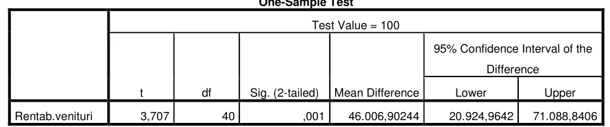
One-Sample Test

Test Value = 100

t df Sig. (2-tailed) Mean Difference

95% Confidence Interval of the

Difference

Lower Upper

Rentab.venituri 3,707 40 ,001 46.006,90244 20.924,9642 71.088,8406

Table 3. The test result variable t on profitability total revenues

The first table is descriptive variable under review and are common elements on:

• N = number of cases analyzed (41); • Mean = average;

• Std.deviation = standard deviation;

• Std.Error Mean = standard error of the mean

The second table shows the actual results of the test, the following notations:

• The variable name = return on total income;

• t = 3707 t test calculated value indicating that the value itself be construed in any way;

• DF = degrees of freedom calculated as N-1 to be reported when the sample size is not

mentioned;

• Sig. (2-tailed) = probability associated with the calculated value of t, which is usually

denoted by "p". In our case p = 0.001 which means that the theoretical distribution of 0,001 t there is a probability of obtaining by chance a value of t equal to or greater than 3.707. Comparing the calculated value of p with the materiality threshold of 0.05 the null hypothesis is accepted, ie, between the two areas there is a significant difference;

• Mean difference = 46006.90244 media is the difference between the sample and the

reference value;

• 95% confidence interval of the difference = show the limits of the confidence interval

for the difference between the sample mean and the reference value. Basically, we can say that in 95% of cases there is a chance that the true difference between the value obtained on the sample and the reference value (100%) to be in the range [20924.9642; 71,088,8406]

Proceeding further to analyze the correlation between total revenue and profitability results in order to understand the degree of involvement of these variables on firm performance and how they influence each other, we get the following:

One-Sample Statistics

N Mean Std. Deviation Std. Error Mean

Table 4. Panel reantabilitatea correlation between total revenues and results

We consider as very suggestive graphical representation using histogram in Figure No.1.

Figure 1. Correlation between average income, total income and profitability results

The graph shows a very strong direct correlation between the three elements taken into account, namely revenues, results and return on total revenue.

b) If the correlation turnover - return on resources consumed

Table 5. Descriptive picture of the profitability variable resources consumed

Correlations

Rezultate Rentab.venituri

Rezultate Pearson Correlation 1 ,409**

Sig. (2-tailed) ,008

N 41 41

Rentab.venituri Pearson Correlation ,409** 1

Sig. (2-tailed) ,008

N 41 41

**. Correlation is significant at the 0.01 level (2-tailed).

One-Sample Statistics

N Mean Std. Deviation Std. Error Mean

Table 6. The test result variable t on profitability resources consumed

Comparing with the previous results, we note that they are close and show the same trend indicating that the probability of obtaining by chance a value of t equal to or greater than 3.269 is slightly increased in this case (0.002), and the chance that the true difference between the value obtained on the sample and the reference value (100%) is in the range [23978.4694; 101656.9453] given the vulnerability expenses.

Correlation we watched it refers to the intensity and direction of concomitant variation between the two variables, one to the other. As can be seen, the values of a variable are in direct sense, breeder, ceilelalte variable values, which means that the two variables are correlated with each other and in one case and another.

Furthermore, analyzing the correlation between turnover and profitability consumption, we get:

Table 7. Panel correlation between turnover and profitability consumed resources profitability

As noted, content following tables 4 and 7, we see that in both cases the correlation is redundant because the picture shows the same correlations twice (above and below the table diagonal) correlations with themselves being perfect and positive (r = 1) . If the second case is very little direct correlation (r = -0.105), it is significant (p = 0.539), in the first case the correlation coefficient = 0.409 Person but the significance is lower (p = 0.008).

Suggestively, as in the previous case, we present in Figure 2 histogram correlation between average turnover, results and profitability of resources consumed.

One-Sample Test

Test Value = 0

t df Sig. (2-tailed)

Mean

Difference

95% Confidence Interval of the

Difference

Lower Upper

Rentab.res.cons 3,269 40 ,002 62.817,70732 23.978,4694 101.656,9453

Correlations

CA Rentab.res.cons

CA Pearson Correlation 1 -,105

Sig. (2-tailed) ,514

N 41 41

Rentab.res.cons Pearson Correlation -,105 1

Sig. (2-tailed) ,514

Figure 2. Correlation between average turnover, results and profitability of resources consumed

Graph submitted to suggest that the profitability of resources consumed shows a very strong correlation with turnover and, all along that automotive sector is the largest generator of expenditure which justifies the direction towards which our research.

CONCLUSION

The analysis carried out confirms the assumption that medium-term prospects remain favorable automotive sector

Anthony R., Govindarajan V., (2007) Management Control Systems, Chicago, Mc-Graw-Hill IRWIN

Charlot, X., (2006) Analyse Fonctionnelle – La Londe les Maures,

http://www.in2p3.fr/actions/formation/ConduiteProjet06/doc-Charlot.pdf

FIELD, A., (2005) Discovering Statistics Using SPSS, Thousand Oaks: Sage Publications

Hilton, R.H., Maher, M.W., Selto, F.S. (2003) Cost Management-Strategies for Business Decision, McGraw Hill Irwin

Iacob, C. (2007) Present and Perspectives in Management Accounting, International Conference Series (II) The Future of Accounting and Accounting profession, Istanbul Commerce University

Jacoby, W.G. (1997) Statistical Graphics for Univariate and Bivariate Data, Thousand Oaks: Sage Publications