Some Explicit Formulae for the Hull and
White Stochastic Volatility Model
Lorella Fatone1, Francesca Mariani2, Maria Cristina Recchioni3, Francesco Zirilli4 1Dipartimento di Matematica e Informatica, Università di Camerino, Camerino, Italy
2Dipartimento di Scienze Economiche, Università degli Studi di Verona, Verona, Italy 3Dipartimento di Management, Università Politecnica delle Marche, Ancona, Italy 4Dipartimento di Matematica “G. Castelnuovo”, Università di Roma “La Sapienza”, Roma, Italy Email: [email protected], [email protected], [email protected], [email protected]
Received November 27, 2012; revised December 29, 2012; accepted January 10,2013
ABSTRACT
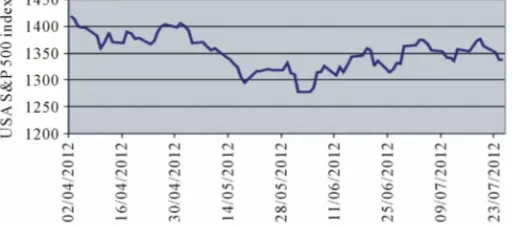
An explicit formula for the transition probability density function of the Hull and White stochastic volatility model in presence of nonzero correlation between the stochastic differentials of the Wiener processes on the right hand side of the model equations is presented. This formula gives the transition probability density function as a two dimensional integral of an explicitly known integrand. Previously an explicit formula for this probability density function was known only in the case of zero correlation. In the case of nonzero correlation from the formula for the transition prob- ability density function we deduce formulae (expressed by integrals) for the price of European call and put options and closed form formulae (that do not involve integrals) for the moments of the asset price logarithm. These formulae are based on recent results on the Whittaker functions [1] and generalize similar formulae for the SABR and multiscale SABR models [2]. Using the option pricing formulae derived and the least squares method a calibration problem for the Hull and White model is formulated and solved numerically. The calibration problem uses as data a set of option prices. Experiments with real data are presented. The real data studied are those belonging to a time series of the USA S&P 500 index and of the prices of its European call and put options. The quality of the model and of the calibration proce- dure is established comparing the forecast option prices obtained using the calibrated model with the option prices actu- ally observed in the financial market. The website: http://www.econ.univpm.it/recchioni/finance/w17 contains some auxiliary material including animations and interactive applications that helps the understanding of this paper. More general references to the work of the authors and of their coauthors in mathematical finance are available in the website: http://www.econ.univpm.it/recchioni/finance.
Keywords: Stochastic Volatility Models; Option Pricing; Calibration Problem
1. Introduction
We study the Hull and White stochastic volatility model [3] in presence of a (possibly) nonzero correlation be- tween the stochastic differentials of the Wiener processes appearing on the right hand side of the model equations.
Let and be respectively the set of real and of positive real numbers and let t be a real variable that de- notes time. The real stochastic processes
, , t t
S V t
, ,
t t
S V
, describe respectively the asset price and the associated stochastic variance as a function of time. The Hull and White stochastic volatility model assumes that
, satisfy the following system of stochastic differ- ential equations (see [3]):
t
dStr S ttd V S W tt td ,t ,
,
(1)
dVt V ttd V Z ttd ,t (2)
where r, ,
t
are real parameters. The processes , ,
t t
W Z 0
, are standard Wiener processes such that
0 0
W Z , and d , , are their stochastic
differentials. Moreover we assume that: d ,
t t
W Z t
d dt t
d , ,E W Z t t (3) where E
denotes the expected value of · and the quantity
1,1
is a constant called correlation co- efficient. The autocorrelation coefficients of the previous stochastic differentials are equal to one.Equations (1) and (2) are equipped with the initial con- ditions:
0 0,
S S (4)
0 0,
V V (5) where 0, 0 are random variables that we assume to be concentrated in a point with probability one. For
simplicity we identify the random variables 0, 0
with the points where they are concentrated. We assume
0, 0 . The assumption 0, 0 with prob-
ability one and (1) and (2) imply that , with probability one for .
S
0
V
S V 0 S V 0
t
S Vt
t
For later convenience we rewrite Equations (1) and (2) using the volatility process vt, , instead of the
variance process t ,
t
V t . Recall that we have: , . Equations (1) and (2) become:
2
t t
V v t
dSt r S t v S W ttd t td ,t ,
(6)
2
d d d ,
2 2
t t t t
v v tv Z t
, (7)
where 2. Note that when r0 and 2 the
Hull and White model (6), (7) reduces to the lognormal SABR model [4]. The lognormal SABR model is a gen- eralization of the Black model in the context of stochastic volatility and is widely used in the practice of the finan- cial markets.
Let us introduce the centered log-return
0
t ln te rt
x S S , t, and the quantity 21
.
Equations (6) and (7) can be rewritten as follows:
2
d d d ,
2
t
t t t
v
x t v W t , (8)
2
d d d ,
2
t t t t
v v tv Z t
, (9)
and the initial conditions (4) and (5) become:
0 0 0,
x x (10)
0 0 0,
v v V (11)
where x0, 0 are random variables that are concen-
trated in a point with probability one. Note that 0
v
x is concentrated in zero with probability one. Moreover the assumption that with probability one and (7) or (9) imply that 0 with probability one for
v
0
t
v t.
The Hull and White stochastic volatility models (1)-(5) has been introduced in mathematical finance in 1987 (see [3]) and is one of the first stochastic volatility models where a diffusion term that is time-varying and stochastic rather than being simply a constant is used to model the variance. More precisely in the Hull and White model a one factor model (i.e. Equation (2)) is used to model the variance (or the volatility) of the asset price (i.e. Equa- tion (2) or (7)). When 0 the transition probability density function of the Hull and White model and the corresponding European call and put option prices have been expressed with closed form formulae. In fact in [3] for the Hull and White model when 0
T
it is shown that the price under a risk neutral measure at time t of a European call option with maturity time , such
that t T , is given by the standard Black Scholes option pricing formula replacing the variance coefficient of the Black Scholes formula with an integrated average sto- chastic variance Vt, 0 t T , where
V 1 T
dT t
t
t V
, 0 t T, and taking the expected value of the resulting formula (see formula (8) in [3]). Note that in [3] no analytical expression for the probabil-ity distribution of the average stochastic variance Vt,0 t T , is given. Only recently when 0 a for-mula for the probability distribution of the average sto-chastic variance Vt, 0 t T
0
, has been deduced [5]. Moreover in [5] when closed form formulae for European call and put option prices in the Hull and White model are given. Until now in the Hull and White model when 0 the option prices have been com- puted using the Monte Carlo method (see [3,5-7]) or evaluating numerically series expansions in the correla- tion coefficient (see, for example, [8]).
In the last decade several modified versions of the Hull and White model have been proposed (see [8-11]). Some of these models contain a multifactor model of the asset price variance (or volatility). Usually in these models the characteristic function of the stochastic process implicitly defined by the model equations can be written explicitly (see, for example, [10,11] and the references therein). Models with nonzero correlation coefficients have been considered. However in these models the dependence of the asset price process from the “volatility process (or processes)” is substantially different than the dependence of these processes in the Hull and White model [3]. Gen- eralizations of the Hull and White model (see, for exam- ple, [9]) in the context of jump diffusion models have also been considered. These generalizations usually re- tain the analytical treatability of the case 0 of the Hull and White model.
In this paper when
1,1
a formula for the tran- sition probability density function associated to the proc- esses x v tt, ,t
, implicitly defined by (8)-(11) is de- duced. This formula gives the transition probability den- sity function of the stochastic processes x v tt, ,t , as a two dimensional integral of an explicitly known inte- grand and its deduction is based on some recent results on the Whittaker functions [1]. The formula obtained generalizes similar formulae deduced recently for the SABR and multiscale SABR models [2]. Thank to it when
1,1
closed form formulae for the prices under a risk neutral measure of European call and put options in the Hull and White model and closed form formulae for the moments of St , t , and of
ln
t St t
dimensional integrals of explicitly known integrands. The closed form formulae for the moments of t ,
, do not involve integrals and have been derived using a technique introduced in [12,13] in the study of the SABR model.
t
The moments of St, t
, are also studied with the same technique, however for these last moments closed form formulae (that do not involve integrals) are avail- able only for the moments of order smaller than two. The moments of t, , of order greater or equal than
two are expressed by formulae containing integrals of ex- plicitly known integrands. Proceeding as done in [12,13] it is possible to use these moment formulae to study cali- bration problems for the Hull and White model when asset price data are considered.
S t
In Section 3 proceeding as done in [14] we show that for the Hull and White model admits infinitely many risk neutral measures depending on a parameter. The risk neutral measures have the same expression of the physi- cal measure when we interpret r as the risk-free interest rate and 2 2
as a new drift that contains the risk pre- mium parameter. This fact makes possible to deduce the option pricing formulae in a risk neutral context.
The results announced are based on the relation of the transition probability density function of the Hull and White model with the “heat kernel” of the index Whit- taker transform [15]. The heat kernel of the index Whit-
taker transform , , is defined as
follows:
1 2
,
h y y , ,y y1 2
2
1 2
2 2 0 1
, 1
π h y
y
c b
W
,i 1 ,i 2
1 2
d sin h 2π e
1 1
i i
2 2
, , , , ,
b b
y
c c W y W y
y y
(12)
where is the set of complex numbers, and i, sinh,
,
, denote respectively the imaginary unit, the hyperbolic sine, the Whittaker function of indices
,
(see [16] page 505) and the gamma function (see [16] page 253). Let and be the real part of b, in [17] it has been shown that a sufficient condition to guarantee the convergence for of the inte- gral contained in (12) is
b Re
b, ,
y y1 2
Re b 2m1 2, m0,1,. The kernel of the index Whittaker transform (12) gen- eralizes the heat kernel of the Kontorovich-Lebedev transform [18,19] that has been used in [2] to derive the explicit formulae of the transition probability density functions of the normal and lognormal SABR and mul- tiscale SABR models.
Let be the Hilbert space of the func-
tions defined on that are Lebesgue square integr-
able in
2 , 2d
L x
x
with respect to the measure x2dx. In our
analysis of the Hull and White model we deduce the fol- lowing formula (see Appendix A):
2 0
,i 2 ,i
0
2 2
1 d sinh 2π 1
2 π
1 d
2
, , , d .
b b
f y b
x
b W y f x
x
y b f L x x
i
i W x,
(13)
Note that the integrals contained in formula (13) must be interpreted in the sense of distributions. Formula (13) is a straightforward consequence of the result presented in [1] and generalizes the inversion formula for the Mac- donald transform presented in [20] and used in [2]. In [1] no restrictions on b are considered. Note that the condi- tion Re
b 1 2 is a sufficient condition to guaranteethe regularity of the functions 1 i
2 b
,
1 i
2 b
,
, (see [17] for further details) that appear in (13).
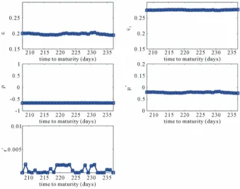
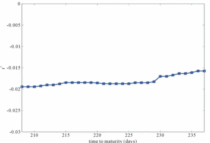
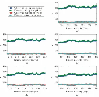
Finally using the option pricing formulae deduced a calibration problem for the Hull and White model (1), (2) is formulated as a nonlinear constrained least squares problem and is solved numerically. The calibration prob- lem considered uses as data a set of option prices. Given the asset prices the calibrated model is used to forecast option prices. Numerical experiments with real data are presented. The real data studied are those belonging to a time series of the USA S&P 500 index and of the prices of its European call and put options. In particular forecast option prices obtained using the calibrated model are compared with the option prices actually observed in the financial market. This comparison establishes the quality of the model and of the calibration procedure.
The website: http://www.econ.univpm.it/recchioni/fi- nance/w17 contains some auxiliary material including animations and interactive applications that helps the un- derstanding of this paper. A more general reference to the work of the authors and of their coauthors in mathe- matical finance is the website: http://www.econ.univpm. it/recchioni/finance.
The remainder of the paper is organized as follows. In Section 2 when
1,1
we derive a formula for the transition probability density function of x v tt, ,t S
t
. In Section 3 we deduce a closed form expression for the first two moments of t, , and an integral repre- sentation formula for the higher moments of t,
S t
of t, . In Section 5 we derive formulae for the
option prices in the Hull and White model. The formulae
deduced in Sections 2-5 hold when . In Sec-
tion 6 using the previous option pricing formulae we formulate a calibration problem for the Hull and White model. Moreover we present a forecasting procedure that, given the asset price at the time of the forecast, forecasts option prices using the calibrated model. The calibration problem and the forecasting procedure are tested in nu- merical experiments with real data. The real data studied are those belonging to a time series of the USA S&P 500 index and of its European option prices. Finally Section 7 is made of two Appendices that contain some auxiliary formulae used in the paper.
t
MN
1,1
backward Kolmogorov equation associated to (8), (9) is invariant by time translation and that this implies that p is a function of s t t instead of being a function of t and t separately when , . We denote with
, 0
t t t t
, ,v s
pMN
x,v t x v, , , ,
MN
p x t ,
x v ,
,s t t , the function MN considered as a func- tion of the variables
p
x v s , ,
. The function pMN
x v s , ,
,
x v ,
, s, satisfies the backward Kolmo- gorov equation associated to (8), (9):
2 2
2 2
2 2 2
2 2
2 2
2 2
,
2 2
, , ,
2
MN MN MN
MN MN
p v p v p v pMN
s x v x v
p p
v
v
x v
x v s
(14)
2. The Transition Probability Density
Function
and the initial condition:
, ,0 , , ,
, ,
MN
p x v x x v v x v
x v
Let us consider the Hull and White models (8)-(11). We denote with p
x v t x v t, , , , ,
,
(15)
v
,v
t,
x , x ,
, , the transition probability density function of the stochastic processes
t0 t t
,
t t
x v , , implicitly
defined by (8)-(11). The function MN
t
, , ,p x v t x , ,v t
where defined as follows: denotes the Dirac’s delta. Recall that ist
is the probability density function of having x x,
given the fact t t
t 2 1.
(16)
x,
vtv, when
v v hat x
x,v ,
x v ,
, t t, 0 , and t t hen 0t we must ch 0 v v0. Note that the
. W
oose x x 0, We show that:
, , , , ,
1 d ei
, , ,
, , , ,
, , 0, ,2π
k x x MN
p x v t x v t x g t t k v v x v x v t t t t
(17) where g is given by:
2 2
2
2 2
ln 2
2 i
8 8
2 1 2 2
1 2 1 2
2
,i ,i
1 e 1
, , , e e e
π 2
1 1
d sinh 2π e i i 2 2 ,
2 2
, , , .
v v
s s k
v v s
a k a k
k v v
k v
a k a k W v k W v k
s k v v
0
g s
(18)Formulae (16), (18) and (19) hold when
1,1
. The functions ν(k) and a(k), k, in (18) are given by:Note that when
1,1
and 0 formula (18) contains the heat kernel of the index Whittaker transform (12) and that when 0 formula (18) can be rewritten as follows:
22
2 2
1 2
i
1 ,
i ,
2
k k
k k
k
a k k
k
,
.
(19)
2 2
2 2 2 ln 2
1 2 1 2
8 8 2 2
i i
2
0
2
, , , e e e d e sinh π ,
π
, , , ,
s s
v v s
v g s k v
s k
iK z
v K k v K k v
v v v v
(20)
where , is the modified Bessel
function of the second kind with purely imaginary index
(see [16] page 375). Moreover when
,z, 0 substituting
2 2 2 2 2 1 2 2 2 2 2 2 2 π 1 2 ln8 2 8 2 2
2 2 1 1 2 cosh 2 2 0 2 0
1 1 1
, , , , , e e e e e
ππ 2
π
d sinh sin e , , , e ,
, , , , , ,0
s s
x x v
s MN
u x x v v vv u
s
v v
p x v t x v t
v s
u
u u q x x u v v
s
x v x v t t t t
, v (21)
where:
0 3 2
2 2 2
2 2 2
2 2
1 1 2
, , , ,
1
1 2 cosh 2 cosh
, , , .
q u v v
v v vv u
v v vv u
u v v
(22)
Formulae (17), (18) and (21), (22) are the main results of this section.
Let us derive formula (18). Substituting (17) in (14), (15) it is easy to see that if the function g satisfies the initial value problem:
2 2 2
2 2
2 2
2
i
2 2 2
i
2
, , , ,
2
,
g v k
kg v g v
s v
g g
k v v
v v
s k v v
g
(23)
0, , ,
, , , ,g k v v vv v v k (24)
Equations (14) and (15) hold. Note that the initial value problem (23), (24) depends on the parameter k and recall that k is the conjugate variable in the Fourier transform of the variable
x x
.Let us seek the solution of problem (23), (24) in the following form:
2 2 2 2 1 i 2 8 2 0 , , ,e e e d e , , ,
, , , ,
k v v d s s s
g s k v v
v L k ,
s k v v
v v (25)
where L is a function that must be determined and (the constant) 1 will be chosen later. Substituting (25) in
(23) it is easy to see that (23) holds if L as a function of satisfies the following equation:
d v
2 2 2 2 2 1 1 i 0, 2 , , , , L L v v v vk v k v d L
k v v
(26)
where and , are given by (16), (19) re- spectively. To solve (26) let us make the following
change of dependent variable:
k k,
1 2
i 2
, , , e , , , ,
, , , .
k v
L k v v v Q k v v
k v v
(27)Moreover in (26) let us consider the new dependent variable Q as a function of the new independent variable
1 22
z k v. Note that the variable z is considered as a complex variable. Let Q z
Q
, , ,k v v
z be the
function Q as a function of . Choosing
2
1 4
d 2 from (26), (27) it follows that Q
satisfies the equation:
2 2 1 2 2i 1 1i i 0,
2 2
Q Q
z z
z z
k Q z
k . (28)
Equation (28) is known as Kummer’s equation (see [16] page 504). The solution of (28) that decays expo- nentially when Re
z is (see [21] page 797):
1 2 i 1 2 1 2
,i , , , e 2 , 0, k v a k
Q z Q k v v
v W k v C k
z z
, , ,v (29)
where C
, ,k v
is a constant with respect to zthat must be determined in order to satisfy the initial condition (24) and a k k
, , is defined in (19).Substituting (29) and (27) in (25) we obtain:
2 2 2
2 2
i 1 2 2 8
i 8 ln 2 1 2
2
2 1 2
,i 0
, , ,
1 e e e e 2
π
d e 2 , , ,
, , , .
s
k v v s v
s a k
g s k v v
k
W k v C k v
s k v v
To impose the initial condition (24) we use formula (24)) (see Appendix A) from which we obtain the fol- lowing expression for C
, ,k v
:
i 1 2 ln 1 2
2 2
1 2 ,i
, ,
1 2 1 e sinh 2π 1 i
2
π
1
i 2 ,
2
, , .
v
a k
C k v
k a k
v
a k W v k
k v
(31) Substituting (31) in (30) we obtain formula (18).
When 0 formula (20) can be deduced from for- mula (18). In fact when 0 we have a k
0, , and the following relations hold (see F. Oberhet- tinger [22] page 287 and [16] page 256, formula 6.1.30):k
1 20,i i , ,
π 2
z z
W z K z
, (32)
1 1 π
i i ,
2 2 cosh π .
(33)
Finally formulae (21), (22) that hold when 0 are obtained rewriting the expression (20) of g when 0 using (32), (33), the formula for the Laplace transform of the function 4
e y
y , y , (see [23], page 146 formula (26)), that follows:
1 2 1 2
4 3 2 1 2 1
0
π
d e e e ,
2
Re , Re 0,
y
zy z
y y z z
z
(34)
and the representation formulae:
1 2 2
i i i
0
1 d e e
2
, , Re , Re , ,
y y
y
K K K y
y
,(35)
cosh i
0
d sin sinh e ,
, Re , .
u
K u u u
(36)Formulae (35) and (36) can be deduced from formula (46) page 35 of [23], formula (9) page 176 of [24], and formula (1.1) of [20] (see [2] for further details).
Note that the technique used here to obtain formulae (17), (18) and (21), (22) is similar to the one used in [2] to deduce the formula for the transition probability den- sity function of the lognormal SABR model.
3. Moments of the Asset Price
Let n0,1,, and Mn be the moment with
respect to zero of the variable , implicitly
defined by (1)-(5), that is:
-n th
, t
S t
0
, , ,
e d e d , , , , ,
, 0, , 0,1, ,
n
n n r t t nx MN
M t t S v
S x vp x v t x
t t t t n
, v t
(37)
where pMN is given by (17) and we have
ln rt
0
e
t
x S
S
and St S,0 t t. Let us rewrite formula (17) as follows:
i, , , , , 1
e d e , , , ,
2π
, , , , , 0, , 0,1, ,
MN
n x x k x x
n
p x v t x v t
k g t t k v v
x v x v t t t t n
(38)
where the functions g nn, 0,1,, will be determined later in this section. Using (38) Equation (37) becomes:
i 0
0
, , ,
e d e d e d e , , ,
e d d , , ,
e , , , 0, , 0,1
n
n n r t t nx nx k x x
n
n nr t t
n
n nr t t n
M t t S v
S x v k g t t k
S k k vg t t k v v
S I t t v t t t t n
, ,
v v
(39)
where
0
, d , 0, ,
n n
I s v vg s v v
, s t t , v ,0,1,
n . That is for n0,1, the knowledge of the
n-th moment Mn of the state variable , is re-
duced to the knowledge of n
, 0
t
S t
I . To determine In we
derive an initial value problem for a partial differential equation satisfied by gn, n0,1,. Note that when
0
n the function g0 is the function g given by (18)
and that the partial differential equation satisfied by g0
that we are looking for is Equation (23).
Substituting (38) in (14), (15) it is easy to see that the functions gn, n0,1,, satisfy the following partial
differential equations:
22 2 2
2
2 2
2 2
2
1 i 1 2
2 2
i ,
2 2
, , , , 0,1, ,
n
n n
n n
g v k n g k n n v g
s
n
g g g
v k n v v
v v
v
s k v v n
(40)
with initial conditions:
0, , ,
,, , , 0,1, .
n
g k v v v v
k v v n
(41)
2 2
2
2 2
ln 2
2 i
8 8
2 1 2 2
1 2 1 2
2
,i ,i
0
1 e 1
, , , e e e
π 2
1 1
d sinh 2π e i i 2 2
2 2
, , , , 0,1, ,
n n
v v
s s k
v v n
n s
n n a k n a k
g s k v v
k v
a k a k W v k W v k
s k v v n
,n (42)
where the functions n
k and a kn
, , are de- fined as follows:k
2 22 2 2
2 2
2
1
2 2
, 2
, , 0,1, ,
n n
n
n n
I n n v I v I
s v
I I
n v v
v v
s v n
2 2
2 2
2 2
2 2
1 1
i 1 2 1 ,
, 0,1, ,
n
n
k n
k
k n
k n
2
(43)
(45)
with initial condition:
0,
1, , 0,1,n
I v v n (46)
1 2
i
, , 0,1,
2 n
n
k n
a k k n
k
(44) It is easy to see that when the solution of
problem (45), (46) is
0,1 n
n
I s v, 1, ,s v . From (39) it follows that:
For when the function gn (i.e. the
function 0,1,
n k0
, 0,
n ,
g s v v ) satisfies problem (40), (41) with k = 0. Integrating with respect to v when v Equa- tions (40), (41) when k = 0, we obtain a set of initial value problems satisfied by the functions In, n0,1,.
That is we obtain the following partial differential equa- tions:
0 , , , 1, 1 , , , e ,
, 0, , , .
r t t
M t t S v M t t S v S t t t t S v
(47)
When problem (45), (46) can be solved using (42) and we have:
1
n
2 2
2
2 2
2 ln
8 8 2
2 1 2 2
0
1 2 1 2
2
0 ,i 0 ,i
0
1 1 1
, e e d e
π 2 0
1 1
d sinh 2π e 0 i 0 i 2 0 2
2 2
, , 2,3, .
n n
s s
v v n
n s
n n a n a
I s v v
v
a a W v W v
s v n
0 ,
n (48)
Substituting formula (48) in equation (39) we obtain the integral representation formula for the moments Mn,
, announced in the Introduction. 2,3,
n
For n2 in order to guarantee that the function gn
does not diverge when v goes to plus infinity and that
0 na is well defined we must require that the real part of n
0 is positive (i.e. Re
n
0
0). This implies that the following condition holds:2 2 2 0.
n n n (49) Condition (49) can be rewritten as a condition for given n, that is:
1 1
1 n , n
n n
1. (50)
For condition (50) guarantees the convergence on the n-th moment n
2
n
M of t, . The same con-
dition for the convergence of the n-th moment of ,
S t
t
S
t , in the case of negative correlation (i.e. the condi-
tion n 1
n
) has been derived in a different 1
way in the study of the lognormal SABR model (i.e. the model obtained choosing r0, 2
2
in (6), (7)) in [25] Theorem 2.3. Note that condition (49) for the con- vergence of the n-th moment can be rewritten as a condition for n given
n
, in this case we have:
2
1 0
1
n .
(51)
From the formula 1
, , ,
e ,r t t
M t t S v S t t , 0,
t t , S v , , and from Equations (6) and (7) it follows that a risk neutral measure of the Hull and White model has the same expression of the physical measure when r is substituted with the risk free interest rate r
and 2 2
is replaced with 2 2 where
2
2
(see [14] Theorem 4.1 and [26], pp. 17-18). That is there are infinitely many risk neutral measures in the Hull and White model depending from the value of the risk pre- mium parameter.
This last observation allows us to interpret the formu- lae derived in Section 5 to price European call and put options under the physical measure as formulae to price these options under a risk neutral measure. Note that calibrating the Hull and White model (1), (2) using asset prices as data we can estimate the parameters of the phy-
sical measure and consequently the pa-
rameters 0
, , , ,
r V
2
,
2
1 and that calibrating
the Hull and White model (1), (2) using option prices as data we can estimate the risk neutral parameters r,
0
, , ,V
. Recall that
0
V cannot be observed in the financial markets and that can be considered as a pa- rameter that must be determined in the calibration pro- cedure. The values of the parameters
,
and obtained in this way determine the value of the risk pre- mium parameter .
4. Moments of the Logarithm of the Asset
Price
The processes ln
e 0
r t
t t
x S S , vt, t
, satisfy Equations (8)-(11) and as a consequence the processes
, , , satisfy the equations:
ln
t S
t vt t 2
d d d ,
2
t
t t t
v
r t v W t
, (52)
2
d d d ,
2
t t t t
v v tv Z t , (53) the initial conditions:
0 0 lnS0,
(54)
0 0 0,
v v V (55) and the assumption (3) on the correlation of the stochas- tic differentials d ,d ,W Z tt t
L
.
For let , be the moment with
respect to zero of 0,1,
n n n th
-t
, t , we have:
0
, , , d d , , , , , ,
, , , 0, 0, 0,1, ,
n n
L t v t vp v t v t
v t t t t n
(56)
where is the transition probability density function associated to the stochastic processes
p
, , t v tt
, im-
plicitly defined by (52)-(55). The function p can be written as follows:
i
1
, , , , , d e , , , ,
2π
, , , , , 0, ,
k x x
p x v t x v t x g t t k v v
x v x v t t t t
(57)and the function g can be determined proceeding as done in Section 2. Note that p depends on s t t and not on and t t separately, , so that we can rewrite the moments of , defined in (56) as follows:
0 t t
, t t
0, , , , ,
i ,
, , , 0,1,
n n
n
n j j j j
L s v L t v t n
D s v j
s t t v n
,,
(58)
where
0 0
d
, d , , ,
d
, , 0,1,
j
j j
k
D s v v g s k v v k
s v j
,
(59)
Proceeding as done in [12,13] in the study of the nor- mal and lognormal SABR models and in Section 3 to deduce the initial value problems (40), (41) and (45), (46)
satisfied by the functions , it is possible
to write an initial value problem satisfied by the function
, , 0,1,
n n
g I n
g and to deduce from it initial value problems satisfied by the functions D jj, 0,1, That is it can be shown that D s v0
,
, s v, , satisfies the following prob-lem:
2
2 2
2
0 0 0
2 , , ,
2 2
D D D
v v s v
s v v
(60)
with the initial condition:
0 0, 1, ,
D v v (61)
and that the functions ,
satisfy the problems:
, , , , 1, 2,
j
D s v s v j
22 2
2 2
2 2
1
2 2
1 1
1
2 2 2
i
i i
2
, , 1, 2, ,
j j j
,
j j
j j
D v D v D j j v
s v v
D
j v j v D jrD
v
s v j
D
(62)
with the initial conditions:
0,
0, , 1, 2, .j
D v v j
(63) Note that in (62) when j1 we set
1 , 0, ,D s v s v .
It is easy to see that the solution of problem (60), (61) is D s v0
,
1, ,s v
. In order to solve the initial value problems (62), (63) let us consider the following change of (independent) variable ln
v , v , and let Dj be the function Dj expressed in the newvariable , that is let D sj
, D sj
,e , s , , j1, 2,. The solutions Dj, j1, 2, of the problems (62), (63) expressed in the variables s ,
2 0
3 2 2 3 2 2
2 1 1
, e d d ,
1 e , i e , ie , i e , ,
2 2
, , 1, 2, ,
s j
j j j
D s s
j j
j D j D D jr D
s j
1j (64)
where
1 2 2 8
2
2 2 22
1
, e e
2π , . , s s s s s s (65)
The integral in the variable in (64) is an elemen- tary integral that can be computed using the following
formula:
4 21 4 2
2 8d , e e e
, .
q q s
q q s s ,
(66)Formulae (64)-(66) together with some elementary computations give:
2 2 2 1 1 11 1 e
i , e , ,
2 1
s s
v
D s v rs s v
,
(67)
2 2 2
2 2
2 2
2
2 1 3 2 2
1 3 3 2
2
6 2
4 5
6 2
1 e 1 e 1 e
, 1 e 2 e
1 2 2
1 e
1 e 1 e
2 5 1 6
s s s s s s s v v
D s v rs
v
3 3 2
3 3 2
s
2 2, , .
2 1 r s s v
(68)
Let us choose , we have in (58),
(67) and (68). It follows that 0
t 0,vv0
s t and that the first three moments of t,t , are given by:
0 0 0 0 0
0 0
, , , 1,
, ,
L t v D t v
t v , (69)
1 0 0 0 0 0 1 0
0 0
, , , i , ,
, , ,
L t v D t v D t v
t v
(70)
2
2 0 0 0 0 0 1 0 2 0
0 0
, , , 2 i , , ,
, , .
L t v D t v D t v D t v
t v
(71)
Proceeding as done to deduce (67)-(71) the expres- sions of the functions D s vn
,
, s , v , and of the moments L tn
, ,v 0 0
, t , ,
0
v0, for can be obtained. These expressions become more and more involved when n increases. Note that formulae (70) and (71) are closed form formulae con- taining only elementary functions of quantities that can be observed in the financial markets. These formulae can be used to formulate calibration problems for the Hull and White model. Thank to the closed form character of these formulae it is possible to develop very efficient nu- merical algorithms to solve these calibration problems. In [12, 13] this idea has been exploited to calibrate the nor-
mal and the lognormal SABR models.
2 n
5. Option Pricing Formulae
Let us derive in the Hull and White model the formulae of the prices at time t0 of European call and put op-
tions having maturity and strike price .
These formulae express the option prices as three dimen- sional integrals of explicitly known integrands.
0
T E0
To this aim we rewrite the transition probability den- sity function (17) as follows:
i , , , , , 1e d e , ,
2π
, , , , , 0, ,
MN
c x x k x x
c
p x v t x v t
k g t t k v v
x v x v t t t t
, , (72)
where c is a constant and gc is a function to be deter-
mined. Let us derive the expression of the function gc.
Substituting (72) in (14), (15) it is easy to see that if gc
satisfies the following partial differential equation:
22 2 2
2
2 2
2 2
2
1 i 1 2
2 2 i , 2 2 , , , , c c c c c
g k c v g k c c v g
s
2 c
g g g
v k c v v
v v
v
s k v v