Estimation of Tree Height and Forest Biomass Using Airborne LiDAR Data: A Case Study of Londiani Forest Block in the Mau Complex, Kenya

http://www.scirp.org/journal/ojf ISSN Online: 2163-0437

ISSN Print: 2163-0429

Estimation of Tree Height and Forest Biomass

Using Airborne LiDAR Data: A Case Study of

Londiani Forest Block in the Mau

Complex, Kenya

Faith Kagwiria Mutwiri

_{, Patroba Achola Odera}

_{, Mwangi James Kinyanjui}

1_{Department of Geomatic Engineering and Geospatial Information Systems, Jomo Kenyatta University of Science and Technology,} Nairobi, Kenya

2_{Division of Geomatics, School of Architecture, Planning and Geomatics, University of Cape Town, Cape Town, South Africa} 3_{School of Natural Resources and Environmental Studies, Karatina University, Karatina, Kenya}

Abstract

Tactical decisions on natural resource management require accurate and up to date spatial information for sustainable forest management. Remote sensing devices by the use of multispectral data obtained from satellites or airborne sensors, allow substantial data acquisition that reduce cost of data collection and satisfy demands for continuous precise data. Forest height and Diameter at Breast Height (DBH) are crucial variables to predict volume and biomass. Traditional methods for estimation of tree heights and biomass are time con-suming and labour intensive making it difficult for countries to carry out pe-riodic National forest inventories to support forest management and REDD+ activities. This study assessed the applicability of LiDAR data in estimating tree height and biomass in a variety of forest conditions in Londiani Forest Block. The target forests were natural forest, plantation forests and other scat-tered forests analysed in a variety of topographic conditions. LiDAR data were collected by an aircraft flying at an elevation of 1550 m. The LIDAR pulses hitting the forest were used to estimate the forest height and the density of the vegetation, which implied biomass. LiDAR data were collected in 78 sampling plots of 15 m radius. The LiDAR data were ground truthed to compare its ac-curacy for above ground biomass (AGB) and height estimation. The correla-tion coefficients for heights between LiDAR and field data were 0.92 for the pooled data, 0.79 in natural forest, 0.95 in plantation forest and 0.92 in other scattered forest. AGB estimated from LiDAR and ground truthed data had a correlation coefficient of 0.86 for the pooled data, 0.78 in natural forest, 0.84 in plantation forest and 0.51 in other scattered forests. This implied 62%, 84% How to cite this paper: Mutwiri, F. K.,

Odera, P. A., & Kinyanjui, M. J. (2017). Estimation of Tree Height and Forest Bio-mass Using Airborne LiDAR Data: A Case Study of Londiani Forest Block in the Mau Complex, Kenya. Open Journal of Forestry, 7, 255-269.

https://doi.org/10.4236/ojf.2017.72016

Received: March 15, 2017 Accepted: April 24, 2017 Published: April 27, 2017

Copyright © 2017 by authors and Scientific Research Publishing Inc. This work is licensed under the Creative Commons Attribution International License (CC BY 4.0).

Keywords

LiDAR, Height, Biomass, Relationship, Correlation

1. Introduction

Forest operations require reliable information on forest status and its evolution

(Ruiz et al., 2014). The main intention of forest inventories is to define the ex-tent, assess the composition and condition of forest resources to ensure sustain-able forest management, which calls for an up to date forest inventory. Forest inventory estimation begun in the middle ages (McRoberts et al., 2010). Timber users (Loetsch & Haller, 1973; Davis et al., 2001) conducted the initial forest in-ventories, focused on estimating growing stock volume. The role of forest have changed over time altering the demands of forest information and hence broa-dening the scope of National Forest Inventory.

The manual methods of forest inventories involved consumed time and cost, as an aid to this the Remote Sensing technology has been used. This technology has been used in various applications around the world: natural resource man-agement (forest ecosystem manman-agement) for many years (Chen et al., 2005), mapping, modeling and understanding of the ecosystem (Lefsky et al., 2002)

among others. Conventional applications of remote sensing used images from passive sensors (Goward & Williams 1997) though topographical covers and weather condition influence them. In few cases, RADARSAT, obtained from ac-tive radar sensors, has been used (Waring et al., 1995).

Light detection and Ranging (LiDAR), also known as Laser altimetry is an ac-tive remote sensing technique that is similar to radar but uses laser light pulses instead of radio waves (NOAA Coastal Services Center, 2012) has been used to minimize the challenges. This technology determines ranges (distances) by tak-ing the product of the speed of light and the time taken for an emitted laser to travel to a target object. The elapsed time from when a laser is emitted from a sensor and intercepts an object can be measured using either; pulsed ranging, or continuous wave ranging, where the phase change in a transmitted sinusoidal signal produced by a continuously emitting laser is converted into travel time

(Lim et al., 2003).

forestry, LiDAR remote sensing has been used in estimating forest attributes such as stand heights, biomass, crown cover density, ground elevation below the forest canopy among others. LiDAR systems produce point clouds representing the height distribution of the forest canopy, which enables one to obtain differ-ent characteristics of a complex forest stand and provide valuable information. This has led to a successful creation of forest inventories at reduced costs (Ruiz et al., 2014). In Kenya, Kinyanjui et al. (2015) demonstrated that LiDAR data can be used to classify the montane forests to show height variations among agro climatic zones and human use zones. However, their work was not ground truthed and gave an estimate of tree heights in the different forests. This study was done in Londiani forest block of the Mau Ecosystem with the objective of testing the applicability of using LIDAR data in developing forest inventory data for Kenya to ease the process of collecting data using conventional forest inven-tory techniques which are time consuming and costly.

2. Methods

2.1. Study Area

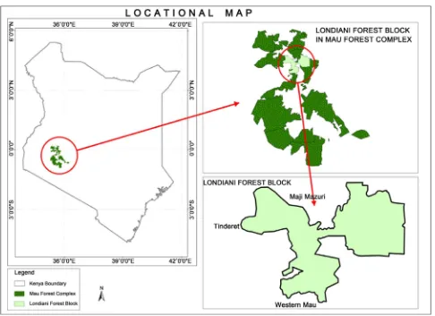
The Mau Forest Complex which covers approximately 400,000 Ha forms the largest closed canopy forest ecosystem in Kenya (Kinyanjui et al., 2014). This complex with a variety of montane forest vegetation is subdivided into 22 blocks. Londiani forest block, one of the blocks, covers an approximate area of 18,938 hectares and Nakuru, Kericho and Baringo Counties. Figure 1 shows the study area which is located between 35˚31'58"E, 35˚46'50"E, and latitudes 0˚10'30"S, 0˚0'10"N. The forest block borders Tinderet, Maji mazuri and Western Mau for-est blocks of the Mau complex.

Londiani Forest block is a montane forest which ranges from 2000 m to 2900 m ASL. The Average temperatures are between 8.6˚C and 23.31˚C. The area has two rainy seasons; the long rains occurring in the months of March to May with average rainfall level of 750 mm and the short rains in October to December with an average rainfall of 423 mm. The driest months are January to February and August to September.

2.2. Data Acquisition

Data sets used in this study include ALS LiDAR data, Aerial image and Ground data from field measurements. The LiDAR data and the Aerial image were cap-tured in February 2014 with a scanner on flight of altitude 1550 m above ground level, point density 2 pts/m2 _{in nadir and the ground sample distance 12 cm.} This data was used to generate the Canopy Height Model (CHM), Digital Sur-face Model (DSM) and the Digital Elevation Model (DEM) for the study area.

2.3. Sampling Design

Figure 1. The location of Londiani Forest Block.

The allocation and selection of sampling plots was based on the elevation, forest cover types and differences in tree heights.

a) Image classification

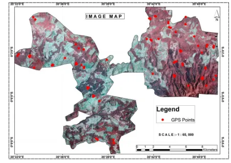
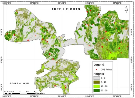
The infrared aerial image (Figure 2) was classified into four forest cover classes namely; natural forest, Plantation Forest, and the other scattered forest (Figure 3). Sample plots were located in each of the classes.

b) Topography /Elevation

Digital Elevation Model was stratified using heights above sea level where sample points were placed within an interval of 200 m, categorizing them into high and low elevation. Low elevation falling between 2000 m to 2400 m and high elevation between 2400 m to 2800 m above sea level (Figure 4).

c) Canopy Height

Figure 2. Aerial image used in the classification.

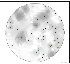
Figure 4. Digital Elevation Model (m), black dots represent the GPS points.

2.4. Field Data Collection

The biometric field data was manually collected using the ICFRA approved me-thodology (REF) for field inventories in Kenya in the period January-April 2015. A circular plot with a radius of 15 m equivalent to the one of the generated grid size of 26.5 × 26.5 m was used. The aim of field measurements was to capture (i) the actual forest heights (ii) the total amount of woody vegetation (biomass) on the sample plots. All trees within the sample plot with diameter at breast height (DBH) of at least 5 cm were measured. Parameters taken for each tallied tree were Diameter at Breast Height (DBH) and the species type. For the sample tree, which was the fifth tree additional features such as Bole height, total height, Stamp height, stamp diameter, species and the tree health, were recorded. The parameters were to aid the estimation of the forest biomass. In total, data was collected from 78 plots.

2.5. Data Processing

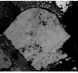
The LiDAR output had infrared image (Figure 6) and point cloud data. The ALS LiDAR point cloud data in las file format, 2.5 × 2.5 km blocks in the Kenyan coordinate system (Arc 1960/UTM zone 37 s), was classified as ground, noise and unclassified; heights were calculated above the reference ellipsoid. LiDAR data processing was performed using lastools (http://rapidlasso.com/lastools/). A Digital Canopy model (DCM) was generated from the first returns (Figure 7). The individual tree positions and heights were extracted from the DCM by ap-plying watershed delineation method where the tree picks become “ponds” and the tree branches/crowns become watersheds for all the sample plots (Figure 8).

Figure 6. Aerial Photograph.

Figure 8. Extracted tree positions.

2.6. Data Analysis

2.6.1. Tree Height Estimation

Tree heights from field observation, were measured only from the sample trees while the diameters at breast heights were measured for all the counted trees in the sample plot. Lauri Mehtätalo’s lmfor-package in R software (Mehtätalo,

2008) that uses the Curtis model was used to estimate unmeasured tree heights.

The model used the measured heights and diameters at breast height measured for the estimation and compared the results with LiDAR data. Curtis model: h (d) = bh + a (d/(1 + d))b_{, Where, h = tree height d = tree diameter at breast} height bh = breast height and a, b= parameters of the equation generated by fit-ting a linear model.

Tree heights from LiDAR data were extracted from the Canopy Height Model (CHM) using plot center coordinates with a radius of 15 m., where heights be-low 2 m were excluded. This was the plot radius where all measurements were taken. The extracted values were then averaged to obtain average tree height in the plot from LiDAR.

2.6.2. Above Ground Biomass (AGB) Estimation

The AGB for each sample plot was calculated using allometric equations

(Ketterings et al., 2001) sourced from Kinyanjui et al. (2014) who interrogated a variety of allometric equations from different sources in Kenya using dummy values for a realistic and unbiased biomass estimation.

The Above Ground Biomass (AGB) of the individual trees was estimated us-ing field measured tree heights and the Diameter at Breast Height (DBH). The ABG for the trees was calculated as follows,

i) Indigenous trees AGB = exp(2.18435 * log10(D1.3)) − (0.20922 * log10(D1.3)) − 1.13559) (Bradley 1988).

ii) Other trees

(

(

( )

)

)

AGB=e ∗ d h − (Chidumayo, 2012) (where AGB—

Above Ground Biomass, D1.3—Diameter at Breast Height at 1.3 m and H— Height.

The Total plot level AGB was calculated from the tree-level biomass values per hectare using R Statistical tool.

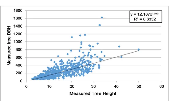
Figure 9. Scatter plots for relationship between measured parameters of Dbh and height.

(Figure 9). The LiDAR estimated AGB was then calculated using the estimated

DBH and the generated tree heights from the Canopy Model. The same models (Allometric equations) used in the estimation of AGB in the field data were used to ensure harmony of AGB estimates. The Total plot level AGB was calculated from the tree-level biomass values per hectare and were therefore compared with the estimation from field data.

2.7. Statistical Analysis

Single factor analysis of variance (ANOVA) at 95% confidence level, correlation and regression analysis were subjected to the data. Scatter plots from the rela-tionships between the two set of variables and the difference in means were gen-erated. The first was the relationship between tree measurements from the ground (field measurements) and trees estimated from LiDAR and the second set of variables was the biomass estimated from field measurements and that from LiDAR. The ground-based data (biometric data) was used as check for the ALS data to determine the usage of the ALS in estimating the height and bio-mass in absence of the ground data. The statistical analysis results were used to evaluate the accuracy based on Root Mean Square Error between the variables under different conditions namely different topographic heights, different ca-nopy heights and different forest cover heights. The same evaluation was done under different topographic conditions to ensure that no bias in LiDAR height and AGB estimates are attributed to slope conditions in a forest.

3. Results

3.1. Tree Heights Estimation

elevation areas (Table 2). 3) Canopy Heights

Table 3 shows a summary of the relationship results indicating a better rela-tionship in the taller trees than the short ones.

ANOVA RESULTS:

Tables 4-6 show the results from ANOVA in different forest types, elevation

and canopy heights respectively.

3.2. Above Ground Biomass Estimation

Linear relationships using the AGB results from biometric data and LiDAR data was calculated. A similar analysis to the heights comparison was done for the forest categories, differences in elevation and canopy heights. Tables 7-9 show a summary of the results.

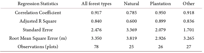
Table 1. Summary statistics for the field height and Airborne LiDAR height (Forest types). Regression Statistics All forest types Natural Plantation Other Correlation Coefficient 0.917 0.785 0.950 0.918 Adjusted R Square 0.840 0.600 0.899 0.836

Standard Error 2.476 3.369 2.079 1.701

Root Mean Square Error (m) 3.350 3.819 2.926 3.265

Observations (plots) 78 25 26 27

Table 2. Summary statistics for the field height and Airborne LiDAR height (Topography). Regression Statistics High Elevation Low Elevation

Correlation Coefficient 0.863 0.955

Adjusted R Square 0.738 0.909

Standard Error 2.908 2.019

Root Mean Square Error (m) 3.688 2.973

Observations 39 39

Table 3. Summary statistics for the field height and Airborne LiDAR height (canopy height). Regression Statistics Height <10 m> 2 m Height > 10 m

Correlation coefficient 0.804 0.840

Adjusted R Square 0.633 0.700

Standard Error 1.258 2.997

Root Mean Square Error (m) 2.862 3.607

Table 4. Summary of Single Factor ANOVA for LiDAR and Field measured heights (Forest types).

Land cover F-calculated F-tabulated Comments

Overall 5.991 3.903 The heights differ

Natural Forest 2.334 4.043 No height difference Plantation Forest 1.481 4.034 No height difference Other land cover 5.384 4.027 Minimal height difference

Table 5. Summary on Single Factor ANOVA for LiDAR and Field measured heights in Different Elevation.

Elevation (m) F-calculated F-tabulated Comments 2000 - 2400 (low Elevation) 2.298 3.967 No difference 2400 - 2800 (High Elevation) 4.019 3.967 Minimal difference

Table 6. Summary of Single Factor ANOVA for LiDAR and Field measured heights in different canopy heights.

Tree Heights (m) F-calculated F-tabulated Comments

2 - 10 26.59724 4.01297 Heights differ

Above 10 4.32675 3.94016 Minimal difference

Table 7. Summary statistics for LiDAR and Field estimated AGB in different forest types. Regression Statistics All forest types Natural Forest Plantation forest Other forest Correlation Coefficient 0.863 0.782 0.839 0.509

Adjusted R Square 0.741 0.594 0.692 0.229

Standard Error 127.441 116.39 168.876 42.301 Root Mean Square Error (m) 206.112 172.75 307.678 62.713

Observations 78 25 26 25

Table 8. Summary statistics for LiDAR and Field estimated AGB in different topography. Regression Statistics High Elevation Low elevation

Correlation Coefficient 0.830 0.899

Adjusted R Square 0.681 0.803

Standard Error 104.304 135.01

Root Mean Square Error (m) 163.602 241.242

Observations 39 39

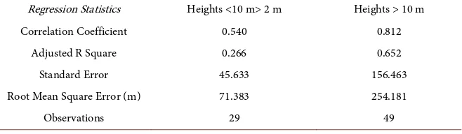
Table 9. Summary statistics for LiDAR and Field estimated AGB in different canopy heights. Regression Statistics Heights <10 m> 2 m Heights > 10 m

Correlation Coefficient 0.540 0.812

Adjusted R Square 0.266 0.652

Standard Error 45.633 156.463

Root Mean Square Error (m) 71.383 254.181

Other land cover 23.14 4.02 Variation in AGB estimated

Table 11. Summary on Single Factor ANOVA for LiDAR and Field estimated AGB in Different Elevation.

Elevation (m) F-calculated F-tabulated Comments 2000 - 2400 (low Elevation) 8.00 3.97 No difference in AGB 2400 - 2800 (High Elevation) 12.39 3.97 Minimal difference in AGB

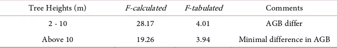
Table 12. Summary of Single Factor ANOVA for LiDAR and Field estimated AGB in different canopy heights.

Tree Heights (m) F-calculated F-tabulated Comments

2 - 10 28.17 4.01 AGB differ

Above 10 19.26 3.94 Minimal difference in AGB

A single factor ANOVA was used to evaluate the variance of the means be-tween the estimated AGB from the estimated heights in the field and LiDAR da-ta. The AGB underwent a similar analysis as the tree height estimates. This was to test if there are any variations in the estimation of AGB under different condi-tions. Tables 10-12 show a summary of the results.

4. Discussions

4.1. Tree Height Measurements

The study assumed that the heights obtained from field measurements were ac-curate and were used to determine the accuracy of estimated heights from Li-DAR data. Several previous studies have indicated a high correlation between tree measurements derived from LiDAR and those measured from the field. However, in this study the correlation was tested under different conditions at a plot level.

The overall correlation of all the plots indicated a high correlation with a value of R2 _{as 0.840, RMSE of 3.350 m and correlation coefficient of 0.917. A further} analysis that was conducted to check the correlation of the estimated heights under different forest types indicated that the plantation forest had the highest correlation with a correlation coefficient of 0.950, a R2 _{value of 0.899 with a} RMSE of 2.926 m. This is in comparison with Natural forest and other forest.

complex shape at the tree-top with overlapping crown, which makes it a chal-lenge to target the tree-top than the plantation forest (Zhen et al., 2016) and may have contributed to the lower correlation as reported.

From the ANOVA results, there was a significance difference in the heights estimated in both high and low elevation areas. However, using the linear re-gression, low elevation areas that were generally flat showed a better correlation than the high-elevated areas. Slope and angle in the hilly (high-elevation) may have contributed this. A study conducted by (Khosravipour et al., 2015), indicate that treetop displacements vary with terrain steepness. A complex slope lowers the accuracy of LiDAR in treetop detection hence the same on CHM generated.

From this study, regression analysis indicate that the height of the trees does not affect the accuracy of LiDAR though there was significance difference using ANOVA in shorter trees.

4.2. Above Ground Biomass Estimation

Field measured AGB was calculated using allometric equation for individual trees then sum of the trees gave plot AGB. DBH used in LiDAR estimation was generated using a model from actual field measurements of DBH and tree height in the field. The two results at a plot level were compared using regression anal-ysis and ANOVA to determine whether there was any relationship or significant variation in the results obtained from both methods.

An overall comparison showed a 0.863 correlation coefficient and a R2 _of 0.741 which indicated a good relationship. However, sorting by forest types gave lower correlations with a R2 _{of 0.692 in Plantation forest and 0.594 in the natural} forest.

Relationships of measured AGB and LiDAR estimated AGB in high and low elevation show a correlation coefficient of 0.830 and 0.899, with a R2 _{value of} 0.681 and 0.803 respectively. A further scrutiny in the canopy height difference, showed poorer relationships in forests with short trees of less than 10 m with a correlation coefficient of 0.54 and R2 _{of 0.27 in comparison to the canopy heights} above 10 m which had R2 _{of 0.65 and a correlation coefficient of 0.81.}

ANOVA results for all the categories show that there is a significant difference in AGB estimation among ground measurements and LiDAR measurements. The difference is attributed to the accuracy of height estimation which has been described as inaccurate in many forestry inventories (Kinyanjui et al., 2015). In addition to this error was propagated into the AGB calculation for LiDAR data because the model used to estimate AGB using ALS was calibrated using ground data.

5. Conclusions and Recommendation

5.1. Conclusions

impor-measurements have to be supplemented with ground data and the best way to use this method would be to complement it with sparse ground data collection points.

5.2. Recommendation

Use of LiDAR with high-density point cloud data would be recommended to improve the accuracy in estimation. This has been proposed world over as a method to enhance the accuracy of LiDAR data (Chen et al., 2005). Secondly, the 15 m radius plot used to confirm the ground data can be tested for accuracy versus costs. A smaller plot provides information at a cheaper cost since the ground trothing team can collect the information over a shorter period. Howev-er, this should be assessed against the ability to capture more accurate informa-tion which might be realized on a bigger plot.

Finally, the availability of the GLAS data for Kenya which covers many forest blocks of Kenya and has many data points (Kinyanjui et al., 2015) should be correlated to this work to find the possibility of estimating biomass on these fo-rests covered by the GLAS data and this would reduce the cost of carrying out a national forest inventory.

Acknowledgements

This study was part of the Improving Capacity in Forest Resources Assessment in Kenya (IC-FRA) project funded by the Finnish Government. It was imple-mented by Kenya Forest Service (KFS) (2010), Kenya Forestry Research Institute (KEFRI), Department of Resource Surveys and Remote Sensing (DRSRS), Uni-versity of Eldoret (UoE), Natural Resources Institute Finland (Luke) and (Fin-nish Forest Research Institute, METLA. The first author is grateful to the Jomo Kenyatta University of Agriculture and Technology for the support granted to her to carry out this research.

References

Chen, C. L, Chiang, T., & Teo, T. (2005). Fusion of LIDAR Data and High Resolution Images for Forest Canopy Modeling.In Proceedings of the 26th Asian Conference on Remote Sensing.

Chidumayo, E. N. (2012). Assessment of Existing Models for Biomass and Volume Cal-culations for Zambia (58 p). Report Prepared for FAO-Zambia Integrated Land Use Assessment (ILUA) Phase II Project.

Press, Inc.

Goward, S. N., & Williams, D. L. (1997). Landsat and Earth System Science: Development of Terrestrial Monitoring. Photogrammetric Engineering and Remote Sensing, 63, 887-900.

Kenya Forest Service (2010). Revised REDD Readiness Preparation Proposal. Kenya. Submitted to the Forest Carbon Partnership Facility. October 2012.

http://www.forestcarbonpartnership.org/sites/forestcarbonpartnership.org/files/Docu ments/PDF/Oct2010/Revised%20RPP%20for%20Kenya.pdf

Ketterings, Q. M., Coe, R., Van Noordwijk, M., Ambagau, Y., & Palm, C. A (2001). Re-ducing Uncertainity in the Use of Allometric Biomass Equations for Predicting Above-Ground Tree Biomass in Mixed Secondary Forest. Forest Ecology and Man-agement, 146, 199-209.

Khosravipour, A., Skidmore, A. K., Wang, T., Isenburg, M., & Khoshelham, K. (2015). Effect of Slope on Treetop Detection Using a LiDAR Canopy Height Model. ISPRS Journal of Photogrammetry and Remote Sensing, 104, 44-52.

Kinyanjui, M. J., Kigomo, N. J., Wambui, K. M., Kariuki, N. J., Charles, N., Macharia, N. J., Odidi, O. W., Fredrick, A., Omamo, O. A., & Katumbi, N. M. (2015). Comparing Tree Heights among Montane Forest Blocks of Kenya Using LiDAR Data from GLAS. Open Journal of Forestry, 5, 80-89. https://doi.org/10.4236/ojf.2015.51009

Kinyanjui, M. J., Latva-Käyrä, P., Bhuwneshwar, P. S., Kariuki, P., Gichu, A., & Wa-michwe, K. (2014). An Inventory of the Above Ground Biomass in the Mau Forest Ecosystem, Kenya. Open Journal of Ecology, 4, 619-627.

https://doi.org/10.4236/oje.2014.410052

Lefsky, M. A., Cohen, W. B., Parker, G. G., & Harding, D. J. (2002). Lidar Remote Sensing for Ecosystem Studies. BioScience, 52, 19-30.

Lim, K., Treitz, P., Wulder, M., St-Onge, B., & Flood, M. (2003). LiDAR Remote Sensing of Forest Structure. Thousand Oaks, CA: Sage Publications.

Loetsch, F., & Haller, K. E. (1973). Forest Inventory, Vol. I. München: BLV Verlagsge-sellschaft.

McRoberts, R. E., Tomppo, E. O., & Næsset, E. (2010). Advances and Emerging Issues in National Forest Inventories. Scandinavian Journal of Forest Research, 25, 368-381. https://doi.org/10.1080/02827581.2010.496739

Mehtätalo, L. (2008). Forest Biometrics with Examples in R. Lecture Notes for the forest Biometrics Course (186 p). http://cs.uef.fi/~lamehtat/

National Oceanic and Atmospheric Administration (NOAA) Coastal Services Center (2012). LiDAR 101: An Introduction to LiDAR Technology, Data, and Applications. Ruiz, L. A., Hermosilla, T., Mauro, F., & Godino, M. (2014). Analysis of the Influence of

Plot Size and LiDAR Density on Forest Structure Attribute Estimates. Forests, 5, 936- 951. https://doi.org/10.3390/f5050936

Waring, R. H., Way, J., Hunt Jr., E. R., Morrissey, L., Ranson, K. J., Weishampel, J. F., Oren, R., & Franklin, S. E. (1995). Imaging Radar for Ecosystem Studies. BioScience, 45, 715-723. https://doi.org/10.2307/1312677

Fair and swift peer-review system

Efficient typesetting and proofreading procedure

Display of the result of downloads and visits, as well as the number of cited articles Maximum dissemination of your research work