Solving nth-Order Integro-Differential Equations Using the
Combined Laplace Transform-Adomian Decomposition
Method
Waleed Al-Hayani
Department of Mathematics, College of Computer Science and Mathematics, University of Mosul, Mosul, Iraq Email: [email protected]
Received February 23, 2013; revised May 1, 2013; accepted May 8, 2013
Copyright © 2013 Waleed Al-Hayani. This is an open access article distributed under the Creative Commons Attribution License, which permits unrestricted use, distribution, and reproduction in any medium, provided the original work is properly cited.
ABSTRACT
In this paper, the Combined Laplace Transform-Adomian Decomposition Method is used to solve nth-order integro-dif- ferential equations. The results show that the method is very simple and effective.
Keywords: Integro-Differential Equations; Laplace Transform Method; Adomian Decomposition Method
1. Introduction
In the recent literature there is a growing interest to solve integro-differential equations. The reader is referred to [1-3] for an overview of the recent work in this area. In the beginning of the 1980’s, Adomian [4-7] proposed a new and fruitful method (so-called the Adomian decom- position method) for solving linear and nonlinear (alge- braic, differential, partial differential, integral, etc.) equa- tions. It has been shown that this method yields a rapid convergence of the solutions series to linear and nonlin- ear deterministic and stochastic equations. The main ob- jective of this work is to use the Combined Laplace Transform-Adomian Decomposition Method (CLT-ADM) in solving the nth-order integro-differential equations.
Let us consider the general functional equation
,
yNy f (1.1) where N is a nonlinear operator, f is a known func- tion, and we are seeking the solution y satisfying (1.1). We assume that for every ,f Equation (1.1) has one and only one solution.
The Adomian’s technique consists of approximating the solution of (1.1) as an infinite series
0
,
n n
y y
(1.2)and decomposing the nonlinear operator N as
0
,
n n
Ny A
(1.3)where An are polynomials (called Adomian polynomi-
als) of y y0, , ,1 yn [4-7] given by
0 0
1 d
, 0,1, 2, ! d
n
i
n n i
n
A N y n
n
.The proofs of the convergence of the series
0 n
n
y
and
0 n
n
A
are given in [6,8-12]. Substituting (1.2) and (1.3) into (1.1) yields0 0
.
n n
n n
y A
f
Thus, we can identify
0
1 0 1
,
, , , , 0,1, 2, .
n n n
y f
y A y y y n
Thus all components of y can be calculated once the
n
A are given. We then define the n-terms approximant to the solution y by
with1 0
n
n i
i
y
y
lim n .
n y y
2. General nth-Order Integro-Differential
Equations
n
b
, m
d
ay x f x y x k x t y t t g x a x b
,1,
(2.1)
with initial conditions
1
0, 1, 2, ,
n
n
y a y a y a y a
where i,i 0,1, , n 1 mn
are real constants, m and are integers and . In Equation (2.1) the functions n
, f x g x
y x
and the kernel are given real-va- lued functions, and is the solution to be deter- mined. We assume that Equation (2.1) has the unique solution.
, k x t
To solve the general nth-order integro-differential Eq- uation (2.1) using, the Laplace transform method, we recall that the Laplace transforms of the derivatives of
are defined by
y x
1
0 1
2
0
0 .
n n n
n n
y x s s y x s s y
s y y
Applying the Laplace transform to both sides of (2.1) and taking into account the fact that the convolution theorem for Laplace transform [13,14] gives:
1 1 0 2 0
, d
, d .
n
n n n
b
m a
b
m a
s y x s s y s y y
g x s f x y x s
k x t y t t s
g x s f x s y x s
k x t s y t t
0
This can be reduced to
1
1 0 2 0 0
1 , d .
n
n n
n n
b
m n
a
y x s
g x s
s y s y y
s f x s s f x s
k x t s y t t
s f x s
(2.2) Substituting (1.2) into (2.2) leads to
0
1
1 2
0
0 0 0
1
, d
n n
n
n n
n n
b
m n n
n a
y x s
The Adomian decomposition method presents the re- cursive relation
0
1
1 2
1
0 0 0
1 , d ,
0,1, 2, .
n
n n
n n
n
b
m n n
a
y x s
g x s
s y s y y
s f x s s f x s
y x s
k x t s y t t
s f x s
n
(2.3) A necessary condition for (2.3) to comply is that
1
lim n 0.
ss f x s
Applying the inverse Laplace transform to both sides of the first part of (2.3) gives , and using the recur- sive relation (2.3) gives the components of 0
y x
, 0n
y x n . We then define the -terms approximant to the solution n
y x by
with1 0
n
n i
i
y x y x
lim n
n y x y x . In this paper, the obtained series
solution converges to the exact solution.
2.1. A Test of Convergence
The convergence of the method is established by Theo- rem 3.1 in [9]. In fact, on each interval the inequality
1 2 2
i i is required to hold for
y y i0,1, , n,
where 0 1 is a constant and is the maximum order of the approximant used in the computation. Of course, this is only a necessary condition for convergence, because it would be necessary to compute
n
2
i for
every
y
0,1, ,
i n in order to conclude that the series is convergent.
2.2. Definition
Let n
x n, 1, 2, be the successive approximations to the solution y x
of a problem. If the positive con- stants K, p exist such that
1
lim n i i ,
p n
n i i
x y x
K
x y x
.
g x s
s y s y y
s f x s s f x s
k x t s y t t
s f x s
then we call the (estimated) Local Order of Conver- gence (EOC) at the point
p
i
x . The constant K is called Convergence Factor at xi.
3. Applications
gro-differential equations is illustrated in the three exam- ples given below. To show the high accuracy of the solu- tion results from applying the present method to our problem (2.1) compared with the exact solution, the maximum error is defined as:
Exact ,
n n
E y x x
where represents the number of iterations. Moreover, we give a comparison among the CLT-ADM, Homotopy perturbation method (HPM) [1] and the varia- tional iteration method (VIM) [2]. The computations as- sociated with the examples were performed using Maple 13 package.
1, 2,
n
Example 1
Solve the second-order integro-differential equation by using the CLT-ADM [1,2]:
1
0
e d
0 1, 0 1
x ,
y x x xty t
y y
t(3.1)
As mentioned above, taking Laplace transform of both sides of (3.1) gives
1
0
ex d
y x s x s xty t t s
so that
1
2
2 2 0
1 1 1
0 0
1 d
s Y s sy y ty t t
s s s
or equivalently
2 4 2
4 1
0
1 1 1 1 1
d 1
Y s ty t t
s s s s s s
where
y x
s Y s
. Substituting the series as- sumption for Y s
as given above in (1.2), and using the recursive relation (2.3) we obtain
0 2 4 2
1
1 4
0
1 1 1 1 ,
1 1
d , 0,1, 2, .
n n
Y s
s s s s s
y x s ty t t n
s
(3.2)
Taking the inverse Laplace transform of both sides of the first part of (3.2) gives y0
x , and using the recur-sive relation (3.2) gives
3 0
3
1
e ,
3!
29 , 1, 2, 3! 30
x
n n
y x x
y x x n
.
Thus the series solution is given by
1
3 1 0
3 1
1
e , 1
3! 30 1
lim lim e e
3! 30
n
x
n i n
i
, 2,
x x
n n
n n
x y x x n
y x x x
[image:3.595.330.516.89.137.2]that converges to the exact solution yExact
x ex. InTable 1, the maximum errors and the EOC are presented for x0.2 0.2 1
n
. Comparing it with the HPM and VIM results given in [1,2], we notice that the result obtained by the present method is very superior (lower error com- bined with less number of iterations) to that obtained by HPM and VIM. From Table 1, it can be deduced that, the error decreased monotically with the increment of the integer .
Example 2
Solve the third-order integro-differential equation by using the CLT-ADM [1,2]:
π2
0
sin d ,
0 1, 0 0, 0 1
y x x x xty t
y y y
t
(3.3)
As early mentioned, taking Laplace transform of both sides of (3.3) gives
π2
0
sin d
y x s xx s xty t t s
so that
3 2
π2
2 2 2
0
0 0
1 1 1
d 1
s Y s s y sy y
ty t t
s s s
0
or equivalently
3 5 3
2
5π2
0
1 1 1 1 1 d
1
Y s ty t t
s s s s s s
where
y x
s Y s
. Substituting the series as- sumption for Y s
as given above in (1.2), and using the recursive relation (2.3) we obtain
0 3 5 3 2
π2
1 5
0
1 1 1 1
, 1 1
d , 0,1, 2, .
n n
Y s
s s s s s
y x s ty t t n
s
(3.4)
Table 1. Maximum error and EOC for Example 1.
x E3 E6 E8 EOC 0.2 1.4815E−06 5.4870E−11 6.0966E−14 0.99999 0.4 1.1852E−05 4.3896E−10 4.8773E−13 1.00000 0.6 4.0000E−05 1.4815E−09 1.6461E−12 0.99999 0.8 9.4815E−05 3.5117E−09 3.9018E−12 1.00000 1.0 1.8519E−04 6.8587E−09 7.6208E−12 1.00000
According to the requirements of our test, 1 2 2
1
i
i
y
y
for all 0,1, 2, , .
Taking the inverse Laplace transform of both sides of the first part of (3.4) gives y0
x , and using the recur-sive relation (3.4) gives
4 0
5 1 5
4
1
cos ,
4!
π 960 π
, 1, 2, 4! 960
n
n n
y x x x
y x x n
.
The series solution is therefore given by
5 1 1
4 1 0
5 1 1
1 π
cos , 1, 2,
4! 960 1 π
lim lim cos cos
4! 960
n n
n
n i n
i
n n
n n
n n
x y x x x n
y x x x x
[image:4.595.309.531.101.276.2] [image:4.595.309.539.463.704.2]that converges to the exact solution yExact
x cosx. InTable 2, the maximum errors and the EOC are shown for
0.2 0.2 1 xn
. Comparing it with the HPM and VIM results given in [1,2], we notice that the result obtained by the present method is very superior (lower error com- bined with less number of iterations) to that obtained by HPM and VIM. From Table 2, it can be concluded that, the error decreased monotically with the increment of the integer .
Example 3
Solve the eighth-order integro-differential equation by using the CLT-ADM [1,2]:
1
8 2 2
0
4 5 6 7
8e d ,
0 1, 0 0, 0 1, 0 2,
0 3, 0 4, 0 5, 0
x
y x x y x x y t t
y y y y
y y y y
6.
(3.5) As previously mentioned, taking Laplace transform of both sides of (3.5) gives
8 2
1 2 0
8e
d
x
y x s x y x s
x y t t s
Table 2. Maximum error and EOC for Example 2.
x E3 E6 E8 EOC 0.2 6.7743E−06 2.1943E−07 2.2297E−08 0.99999 0.4 1.0839E−04 3.5109E−06 3.5676E−07 0.99999 0.6 5.4872E−04 1.7774E−05 1.8061E−06 1.00000 0.8 1.7342E−03 5.6175E−05 5.7082E−06 1.00000 1.0 4.2339E−03 1.3714E−04 1.3936E−05 0.99999
According to the requirements of our test, 1 2 2
1
i
i
y
y
n
for all i0,1, 2, , .
so that
8 7 6 5 4
4 5 6 7
3 2
1
3 3
0
0 0 0
0 0 0 0
8 2 2 d
1
s Y s s y s y s y s y
s y s y sy y
Y s y t t
s s s
0
or equivalently
7 5 4 3 2
8 8 8 8 8 8 8
1
3 8 8 3 8
0
2 3 4 5 6
1 1 1 1 1 1
2 8 2 d
1 1 1 1
Y s
s s s s s s
s s s s s s s
y t t
s s s s s s
1
where
y x
s Y s
. Substituting the series as- sumption for Y s
as given above in (1.2), and using the recursive relation (2.3) we obtain
7 5 4 3 2
0 8 8 8 8 8 8
8 3 8 8
2 3 4 5
1 1 1 1 1 1
6 2 8
1 1 1 1
s s s s s
Y s
s s s s s s
s s s s s
s
(3.6)
1
3
8
1
0
2 d , 0,1, 2, .
1
n n
y x s y t t n
s s
Taking the inverse Laplace transform of both sides of the first part of (3.6) gives y0
x , and using the recur-sive relation (3.6) gives
2 0
2 1
6 2 6
2
6 6
5e 1e e 1cos
4 4 2
2 2
sin sinh ,
2 2
1cos 1cosh sin 2 sinh 2 ,
2 2 2 2
0.5512 10 0.2756 10 cos 0.2756
2 2
10 cosh 0.5512 10 sin sinh
2 2
x x x
y x x x x
x x
y x x x x x x
y x x x
x x
x
12 2 12 3
12 12
18 2 19 4
19 18
,
0.3038 10 0.1519 10 cos 0.1519
2 2
10 cosh 0.3038 10 sin sinh ,
2 2
0.1674 10 0.8371 10 cos 0.8371
2 2
10 cosh 0.1674 10 sin sinh ,
2 2
y x x x
x x
y x x x
x x
x
[2] X. F. Shang and D. F. Han, “Application of the Varia- tional Iteration Method for Solving nth-Order Integro- Differential Equations,” Journal of Computational and Applied Mathematics, Vol. 234, No. 5, 2010, pp. 1442- 1447. doi:10.1016/j.cam.2010.02.020
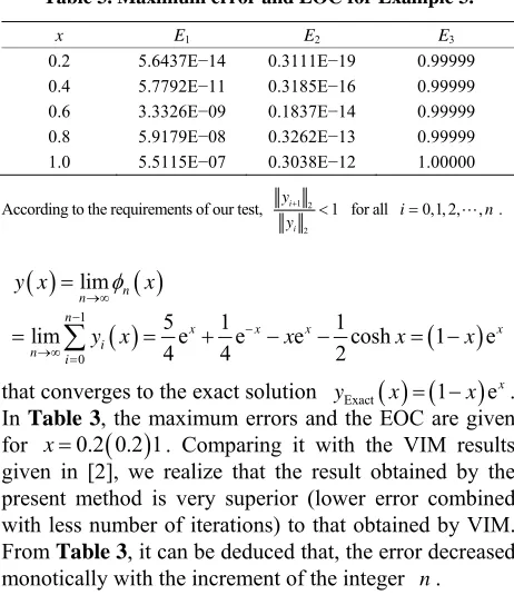
Table 3. Maximum error and EOC for Example 3.
x E1 E2 E3
0.2 5.6437E−14 0.3111E−19 0.99999 0.4 5.7792E−11 0.3185E−16 0.99999 0.6 3.3326E−09 0.1837E−14 0.99999 0.8 5.9179E−08 0.3262E−13 0.99999 1.0 5.5115E−07 0.3038E−12 1.00000
According to the requirements of our test, 1 2 2
1
i
i
y
y
for all i0,1, 2, ,n.
[3] A. M. Wazwaz, “The-Combined Laplace Transform-Ado- mian Decomposition Method for Handling Nonlinear Volterra-Integro Differential Equations,” Applied Mathe- matics and Computation, Vol. 216, No. 4, 2010, pp. 1304-1309. doi:10.1016/j.amc.2010.02.023
1
0
lim
5 1 1
lim e e e cosh 1 e
4 4 2
n n n
x x x
i n
i
y x x
y x x x x
[4] G. Adomian, “Stochastic Systems,” Academic Press, New York, 1983.
[5] G. Adomian, “Nonlinear Stochastic Operator Equations,” Academic Press, New York, 1986.
x
[6] G. Adomian, “Nonlinear Stochastic Systems Theory and Applications to Physics,” Kluwer Academic Publishers, Dordrecht, 1989. doi:10.1007/978-94-009-2569-4
that converges to the exact solution yExact
x 1 x
ex.In Table 3, the maximum errors and the EOC are given for x0.2 0.2 1
. Comparing it with the VIM results given in [2], we realize that the result obtained by the present method is very superior (lower error combined with less number of iterations) to that obtained by VIM. From Table 3, it can be deduced that, the error decreased monotically with the increment of the integer n.[7] G. Adomian, “Solving Frontier Problems of Physics: The Decomposition Method,” Kluwer Academic Publishers, Dordrecht, 1994.
[8] K. Abbaoui and Y. Cherruault, “Convergence of Ado- mian’s Method Applied to Differential Equations,” Ma- thematical and Computer Modelling, Vol. 28, No. 5, 1994,
pp. 103-109.
[9] K. Abbaoui and Y. Cherruault, “New Ideas for Proving Convergence of Decomposition Methods,” Computers and Mathematics with Applications, Vol. 29, No. 7, 1995,
pp. 103-108. doi:10.1016/0898-1221(95)00022-Q
4. Conclusion
The CLT-ADM has been applied for solving nth-order integro-differential equations. Comparison of the results obtained by the present method with that obtained by HPM and VIM reveals that the present method is supe- rior because of the lower error and less number of needed iteration. It has been shown that error is monotically re- duced with the increment of the integer n.
[10] K. Abbaoui and Y. Cherruault, “Convergence of Ado- mian’s Method Applied to Nonlinear Equations,” Mathe- matical and Computer Modelling, Vol. 20, No. 9, 1994,
pp. 60-73. doi:10.1016/0895-7177(94)00163-4
[11] Y. Cherruault and G. Adomian, “Decomposition Methods: a New Proof of Convergence,” Mathematical and Com- puter Modelling, Vol. 18, No. 12, 1993, pp. 103-106.
doi:10.1016/0895-7177(93)90233-O
5. Acknowledgements
[12] S. Guellal and Y. Cherruault, “Practical Formula for Cal- culation of Adomian’s Polynomials and Application to the Convergence of the Decomposition Method,” Interna- tional Journal Bio-Medical Computing, Vol. 36, No. 3,
1994, pp. 223-228. doi:10.1016/0020-7101(94)90057-4 We would like to thank the referees for their careful re-
view of our manuscript.
REFERENCES
[13] A. D. Polyanin and A. V. Manzhirov, “Handbook of In-tegral Equations,” CRC Press, New York, 1998.
doi:10.1201/9781420050066
[1] A. Golbabai and M. Javidi, “Application of He’s Homo- topy Perturbation Method for nth-Order Integro-Differ- ential Equations,” Applied Mathematics and Computation, Vol. 190, No. 2, 2007, pp. 1409-1416.
doi:10.1016/j.amc.2007.02.018
![Table 1. In the error decreased monotically with the increment of the integer Exactfor results given in [1,2], we notice that the result obtained by the present method is very superior (lower error com- bined with less number of iterations) to that obtaine](https://thumb-us.123doks.com/thumbv2/123dok_us/7773112.718092/3.595.330.516.89.137/decreased-monotically-increment-exactfor-obtained-present-superior-iterations.webp)
![Table 2, the maximum errors and the EOC are shown for 0.2 0.2 1results given in [1,2], we notice that the result obtained](https://thumb-us.123doks.com/thumbv2/123dok_us/7773112.718092/4.595.309.539.463.704/table-maximum-errors-shown-results-notice-result-obtained.webp)