A Rough Set Based Optimization Method for Elderly Evaluation

(1)

http://www.scirp.org/journal/ijis ISSN Online: 2163-0356

ISSN Print: 2163-0283

DOI: 10.4236/ijis.2017.72003 Apr. 30, 2017 25 International Journal of Intelligence Science

A Rough Set Based Optimization Method for

Elderly Evaluation

Weiping Li, Tong Mo, Xingzhang Ren, Jingbo Zhang, Zhonghai Wu

School of Software and Microelectronics, Peking University, Beijing, China

Abstract

In order to improve the efficiency of elderly evaluation, an optimization me-thod based on rough set is proposed. Compared with the traditional rough set attribute reduction, the redundant evaluation items are eliminated by items’ correlation. It avoids a big overhead of calculating the core of rough sets that have many attributes. A novel rule reduction method is proposed based on re-liability and coverage, in order to solve the problem of rarely appeared rules and conflict rules in traditional rough set. A sorting algorithm based on cov-erage is used to optimize the traditional flat evaluation questionnaire model with a hierarchical order. By these optimizations, the number of items that need to evaluate is greatly reduced. The proposed approach is deployed in an elderly service company named Lime family. Real-life result shows that the method can reduce more than 40% items with over 90% accuracy prediction rate. Compared with decision tree and the method based on expert knowledge in reduction rate and accuracy rate, the method has same performance in one index, and 20% improvement on average in the other one.

Keywords

Rough Set, Attribute Reduction, Elderly Evaluation, Decision Rule

1. Introduction

The population aging problem is getting serious in China, and the care of the elderly has become a heavy burden on the family. Thus, professional community care and family support for the elderly become more important than ever before. Nursing care service which refers to the professional care team providing daily care service for the elderly and disabled persons is essential in the elderly service. Currently the professional nursing service is developing rapidly in china. To de-liver the nursing service, we need to perform the health evaluation for an elder How to cite this paper: Li, W.P., Mo, T.,

Ren, X.Z., Zhang, J.B. and Wu, Z.H. (2017) A Rough Set Based Optimization Method for Elderly Evaluation. International Jour-nal of Intelligence Science, 7, 25-53. https://doi.org/10.4236/ijis.2017.72003

Received: March 26, 2017 Accepted: April 27, 2017 Published: April 30, 2017

http://creativecommons.org/licenses/by/4.0/

(2)

DOI: 10.4236/ijis.2017.72003 26 International Journal of Intelligence Science person to learn his/her health status. The proper care program for the elderly will be based on the health evaluation. During the implementation of the care program, periodic health evaluation will be performed to evaluate and improve the program. As we can see that the health evaluation of the elderly is one of the important tasks in the nursing service.

There exist some elder evaluation methods which are based on the Barthel Index [1] and the Ability assessment for elder adults [2], with data from ques-tionnaires or face-to-face interviews. Our work is based on the data from the Lime family company, a professional company providing elderly care service in China. Lime family customizes their own evaluation table based on the Chinese Professional Standard MZ/T 039-2013 and Barthel Index. Normally the investi-gator fills the tables on the basis of face to face or telephone interviews. A lot of evaluation items need to be investigated in order to fully understand the status of an elderly person. On one hand, the survey becomes a time consuming task. On the other hand, in the evaluation process we found that some items are re-dundant. After some items are determined, a lot of related items can be esti-mated and the investigator doesn’t need to ask the elderly. For instance, a person with the Alzheimer’s disease normally cannot go outside by himself and hence cannot go out for shopping, for running and so on. To this end, this paper fo-cuses on the reduction of the evaluation items and the sort of the evaluation items to improve and simplify the evaluation process and improve the efficiency.

The key to optimize the evaluation model is to speculate the value of items from some related items in the questionnaire and to sort the items to make the speculation more efficiently. The often used methods for the health and elder evaluation include the actor analysis method in Statistics and Rasch analysis method [3][4]. The main task in these methods is the deletion of the redundant evaluation items. These methods will get a small set of items. But these items are still in a flat model, namely, the dependency among them are not analyzed. Another kind of methods is to analysis the relationship among the items, for example the Bayes method [5], decision tree [6][7], and the frequent pattern mining [8]. To improve the efficiency of the elder evaluation, we need to reduce the items to be asked by speculating them with other items and to sort the items. The attribute reduction in the Rough Set theory provides a way to resolve both questions [9][10][11][12].

As a mathematical tool to deal with these imprecise, inconsistent and incom-plete information and knowledge, Rough set theory has been widely concerned since it was proposed by Professor Pawlak in 1982 [13] [14]. It has been widely used in the field of machine learning, data mining, and decision support

[15]-[20]. Since the rough set theory can effectively deal with the vague and un-certain data without any additional information or a priori knowledge, this pa-per take the Rough Set method to improve the elder pa-person evaluation.

(3)

DOI: 10.4236/ijis.2017.72003 27 International Journal of Intelligence Science conditional entropy of evaluation items; proposes an attribute reduction method for eliminating redundant evaluation items. 2) Proposes the concept of reliability and coverage degree for the decision equivalent class, which promote the rule generation method in the rough set by avoiding the uncertain rule and the rarely appeared rules. 3) Presents an evaluation items sort algorithm based on the cov-erage degree. By this mean, we change the traditional flat evaluation model into an orderly evaluation model. The elderly evaluation process can be carried out in the sorted order and predict some items with the decision rules, which will re-duce the evaluation items that need to be asked upfront.

This paper is organized as follows. Section 2 reviews related work. Section 3 introduces the evaluation attribute reduction method and prediction rule opti-mization method. Section 4 introduces the rough set based model for improving the elderly evaluation and the core algorithms. Section 5 shows the experiment results with the real case data. Section 6 concludes the paper.

2. Related Work

The work in this paper is to optimize the elderly evaluation process. On the one hand, we will analyze the evaluation items to find out the redundant items, which will reduce the workload of the survey. On the other hand, we will esti-mate the uninvestigated items with the known items to reduce the items col-lected from elderly people. This section reviews the item reduction of the healthcare questionnaire; the prediction of related items and the rough set attribute reduction method.

2.1. Item Reduction in Healthcare Question Area

Usually people take the statistics methods to reduce or delete the evaluation items. Luis Prieto take the Exploratory Factor Analysis (EFA) method of the Classical Test Theory (CTT) and the Rasch Analysis (RA) method of the item response theory reduce the Nottingham Health Profile (NHP 38) [3]. The 38 items are reduced to 20 items and 22 items respectively and get the new scale NHP 20 and NHP 22. CTT resulted in 20 items (4 dimensions) whereas RA in 22 items (2 dimensions). Both instruments showed similar characteristics under CTT requirements: item-total correlation ranged 0.45 - 0.75 for NHP20 and 0.46 - 0.68 for NHP22, while reliability ranged 0.82 - 0.93 and 0.87 - 94 respectively.

Ephrem Fernandez uses a 3-setp decision rule to reduce the McGill Pain Questionnaire (MPQ). By using the minimum absolute frequency of 17 and the minimum relative frequency of 1/2 as threshold value, the words of MPQ are reduced from 78 to less than 20 in average. The selective reduction and reorgan-ization of these descriptors can enhance the efficiency of this approach to pain assessment [4].

(4)

DOI: 10.4236/ijis.2017.72003 28 International Journal of Intelligence Science For example, the health of the elderly usually has a strong impact on the ability of self-care. Therefore, the order of items is as important as reducing the number of questionnaire items need to be asked.

2.2. Prediction of Related Items

The values of some evaluation items can be inferred from their high correlation items, so that some items are not need to be asked, and the efficiency of evalua-tion is improved. The related methods include Bayesian formulaevalua-tion, decision tree, and frequent pattern mining and so on.

A Bayesian forecasting model is described in the literature [5], estimating the prior probabilities from a sample of SPEAK Test scores of 803 prospective ITAs at UVa between 2006 and 2013, and using the TOEFL iBT scores from 318 stu-dents to update the forecast probabilities. Overall, this forecasting model de-monstrates and explains a useful statistical association between the SPEAK Test scores and the TOEFL iBT scores, used widely in university admissions.

In the literature [6], S.S. Panigrahi deals with two established technique viz. Epsilon-SVR and Decision Tree for stock market forecasting. The available nu-merical historical data and some technical indices of BSE-sensex have been used for empirical studies. Both epsilon-SVR and Decision Tree techniques are run over the dataset, respective efficiencies has been evaluated and explained through established statistical parameters. The work concludes that the SVM has outper-formed decision tree in training front and lagged behind in validation in com-parison with regression decision tree.

Le Thi Ngoc Anh proposes the forecast model of the possibility of cholera oc-currence in Hanoi city based on association rule mining from cholera dataset collected in Hanoi’s districts from 2001 to 2012 [8]. Experimental results show that the proposed method is suitable for cholera forecast and can be used as an important input in the decision making process of the preventive healthcare.

Chunmei Liu introduces non-financial index into financial risk forecasting system to establish mix financial index evaluation system including financial in-dex and non-financial inin-dex, and also introduces C4.5 decision tree arithmetic into the modeling process [7]. According to the 40 trained listed companies in the 2004, 2005, get the model of “model trained”, its accuracy rate is 82.5%.

2.3. Attribute Reduction Based on Rough Set

(5)

in-DOI: 10.4236/ijis.2017.72003 29 International Journal of Intelligence Science crease the indeterminacy of decisions; 4) the traditional decision rule generation algorithms may generate rarely appeared rules.

Compared with traditional rough sets theory, Honghai Feng uses rule genera-tion algorithm (RGA) to reduce the attributes instead of calculating the core [9]. Experimental results show that RGA achieves good classification performance. In order to improve the efficiency of attribute reduction, Chen yanyun integrates the parallel idea in the attribute reduction and construct a parallel rough set attribute reduction algorithm based on attribute frequency [10]. The algorithm is applied to corn breeding. Experiments show that the algorithm outperforms the traditional algorithms. In the literature [11] Hiroshi Saka and others extend rough set-based rule generation algorithm. They have extended this algorithm to tables with non-deterministic information, and implemented it according to the constraint satisfaction problem. This algorithm is important for rule generation in tables with uncertainties. Zhe Liu provides a new heuristic algorithm named “Short First Extraction (SFE)” based on the classical rough set theory for rules generation [12]. Based on the datasets provided by UCI machine learning repo-sitory, SFE has better performance than Johnson Reducer, genetic reducer and Holte’s 1R reducer. SFE is a new rules generating method.

In summary, using another method instead of calculating the core to reduce the attributes and generate rules is a feasible way. In this paper, we optimize the model of elderly evaluation based on rough set, and information entropy and conditional entropy are introduced in attribute reduction. We also define the re-liability and coverage to optimize the process of decision rules, in order to avoid the problems mentioned above.

3. Problem Formulation

[image:5.595.208.526.526.733.2]

This section provides the definition for rough sets of elderly evaluation model. The notations and description mentioned in this section is shown as Table 1.

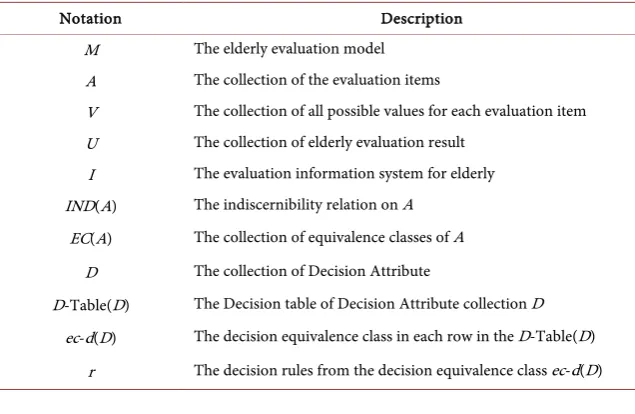
Table 1. Notations and description.

Notation Description

M The elderly evaluation model A The collection of the evaluation items

V The collection of all possible values for each evaluation item U The collection of elderly evaluation result

I The evaluation information system for elderly IND(A) The indiscernibility relation on A

EC(A) The collection of equivalence classes of A D The collection of Decision Attribute

D-Table(D) The Decision table of Decision Attribute collection D ec-d(D) The decision equivalence class in each row in the D-Table(D)

(6)

DOI: 10.4236/ijis.2017.72003 30 International Journal of Intelligence Science

3.1. Definition

Definition 3.1 Let M =

(

A V,

)

be the elderly evaluation model. Where,

(

1, ,2 , m

)

A= a a  a , is the collection of the evaluation items, V is a collection of

all possible values for each evaluation item.

Definition 3.2 Let U be the collection of elderly evaluation result.

Let vi(aj) be the evaluation value of aj of i-th elder person, the evaluation result of the i-th elder person can be ui=

(

v ai

( ) ( )

1 ,v ai 2 ,,v ai

( )

m

)

, then the domain

{

1, 2, , n

}

U = u u  u is the collection of the evaluation result of all persons.

Definition 3.3 Let I=

(

U A V, ,

)

be the evaluation information system for

elderly. Based on the definition 3.1 and 3.2, I can be defined with the Rough set theory.

Definition 3.4 Let IND(A') be the indiscernibility relation on A', which is the collection of the evaluation items. Where A' is the subset of A, A′ ⊆A, if there

exist two elder person p and q, for ∀ai, ai∈A′, we can have that

( )

p i q i

v a =v a , then p and q have the indiscernibility relation, namely IND(A').

Definition 3.5 Let EC(A') be the collection of equivalence classes of A'. For the collection of the evaluation items A′ ⊆A，A′ =

(

a a₁, ₂,,ap

)

, the evaluation result of elderly i ui =

(

v ai

( ) ( )

1 ,v ai 2 ,,v ai

( )

p

)

, and the indiscerni-bility relation on IND(A'), we can get some equivalence classes, ec1(A'), ec2(A'),

, ecq(A'). If the evaluation result in each equivalence classes are equal, while differ with other equivalence classes, then these equivalence classes constitute the collection of equivalence classes EC(A').

Definition 3.6 Decision Relation, Decision Attribute, and Condition Attribute. In the elderly evaluation model, there exists the logic inference relation among items, namely, one item can be determined by other items. If the value of D, col-lection of items, can be inferred by the colcol-lection C, then the collection C have the decision relation on collection D, denote as C→D, C⊆A, D⊆A, CD=ϕ. C is the collection of condition Attribute, and D is the collection of

Decision Attribute.

Definition 3.7 Let the D-Table(D) be the Decision table of Decision Attribute D, and ec-d(D) be the decision equivalence class.

The Decision table of Decision Attribute D, D-Table(D), is composed of the decision relation C→D, condition Attribute C, Decision Attribute D, EC(C),

i.e. the collection of equivalence classes of C, and the eci(C) and the value of de-cision attribute in EC(C). Each row in the table is a decision equivalence class ec-d(D).

Definition 3.8 Decision rule r.

From the decision equivalence class ec-d(D) in the decision table D-Table(D), we can create some decision rules r= prec→posc. Where the post condition

posc is the value of the decision attribute in the same row, precondition prec is the subset of the condition attribute.

(7)

DOI: 10.4236/ijis.2017.72003 31 International Journal of Intelligence Science attribute to build a decision table. Optimize the decision table by finding and eliminating the redundant items. Optimize each decision equivalence class by eliminating those equivalence classes that may create uncertain rules or rules with low support. Create rules according to each equivalence class in the deci-sion table. Calculate the value of the decideci-sion attribute with the condition attributes, which lead fewer items are asked during the evaluation process.

3.2. Calculating the Correlation Degree of Evaluation Items

In turn, one evaluation item will be selected as the decision attribute to build a decision table, left the others as the condition attribute. Normally not all these condition attributes have impact on the decision attribute, so attribute reduction will be performed to eliminate those have weak impact on the decision attribute. The attribute reduction is depending on the importance of the condition attribute on the decision attribute. If there is such an evaluation item in the deci-sion table, when the value of other condition attributes is assigned the decideci-sion attribute will be fixed, despite the change of it. Then apparently this evaluation item has no impact on the decision attribute which should be eliminated.

Thus it can be seen the correlation degree of evaluation items in the decision table is important to the attribute reduction. So we need to calculate the correla-tion degree of evaluacorrela-tion items, which is determined by the condicorrela-tional proba-bility among the attribute values. The conditional probaproba-bility of the evaluation items’ value is, when one attribute is assigned, the probability of the other items take a certain value. It means that the higher conditional probabilities have higher correlation degree of the two items.

The evaluation items have different values. The probability distributions of the values are different from one item to others. For some evaluation items it is uniform distribution for most of the elder persons, but for some other items it may focus on one value, only few people have other values. In section five we have statistics on the data of the experimental persons. From Figure 2 we can see that the probability distributions of different items’ value are different and most of them are not uniform distribution. Given this, one should take into account the probability distribution of the items’ value to calculate the correla-tion of evaluacorrela-tion items. For instance, suppose the condicorrela-tional probability is 100%, namely when item take a certain value, the probability of item B taking a certain value is 100%. But if this value of item B is scarce, namely, only a few people take this value, the corresponding decision equivalence classes have less meaning.

Entropy is a property of thermodynamically systems, which can measure the uniformity of the distribution of objects. Combine the concept of entropy and the conditional probability; we use the concept of conditional entropy in infor-mation theory to discuss the calculation method of correlation degree of evalua-tion items [21].

(8)

( )

_{( )}

1

log

i

i a

x x i

H x P x

P x

∈

=

∑

(1)

where P(xi) is the probability of x take the value xi, and a is an arbitrary value. The conditional entropy of evaluation item x on item y is,

( )

_{( )}

1

log

j i

j i j a

y y x x _i _j

H x y P y P x y

P x y

∈ ∈

=

_∑

₍₂₎

where P x y

( )

is the conditional probability of x take xi when y is yj, a is an

ar-bitrary value.

With H(x) and H x y

( )

, the Correlation degree,

( )

, 1 H x y

( )

_{( )}

H y x

( )

_{( )}

SU x y

H x H y

+ = −

+ (3)

Suppose evaluation item x may be the value of x0x1, y may be the value of y0y1. When x and y are independent of each other, no matter what the value of x is, it has not impact on y, namely, P x y

(

0 0

)

=P x

( )

0 , P x y

(

0 1

)

=P x

( )

0 , ,

(

0 0

)

( )

0

P y x =P y , P y x

(

1 0

)

=P y

( )

1 , , put them into the formula 2, we

have, H x y

( )

=H x

( )

, H x y

( )

=H x

( )

, then put H x y

( )

into formula 3, we

get SU X Y

(

,

)

= − =1 1 0.

When x and y are related, we have P x y

(

0 0

)

<P x

( )

0 , P x y

(

0 1

)

<P x

( )

0 ,

, P y x

(

0 0

)

<P y

( )

0 , P y x

(

1 0

)

<P y

( )

1 , , H x y

( )

<H x

( )

,

( )

H y x <H y , put them into the formula 3 we get SU x y

(

,

)

<1.

When x and y have completely correlation, namely, x = x0, there must exist y = y0 or y = y1, i.e., when x = x0, we have P x y

(

0 0

)

=1 and P x y

(

0 1

)

=0, or

(

0 0

)

0

P x y = and P x y

(

0 1

)

=1.

In the same way, when y = y0, there must exist x = x0 or x = x1, then

(

0 0

)

1

P y x = and P y x

(

0 1

)

=0, or P y x

(

0 0

)

=0 and P y x

(

0 1

)

=1.

With formula 2 we have H x y

( )

=0, in the same way, H y x

( )

=0. Thus, with formula 3, SU X Y

(

,

)

= − =1 0 1.

With formula 3, on the one hand, we can calculate the correlation degree be-tween the condition attributes and the decision attribute and, by setting a threshold, filter the condition attribute whose impact on the decision is lower. On the other hand, we can also calculate the correlation degree of between dif-ferent condition attributes to further filter some condition attribute(s), which actually eliminate some attributes with similar function.

3.3. The Measure of Reliability and Coverage Degree for the

Decision Equivalent Class

(9)

DOI: 10.4236/ijis.2017.72003 33 International Journal of Intelligence Science that the situation for this rule is rare and this rule is a sparse rule that should be eliminated.

The main reason for rule conflict lies in the inconsistent decision table, i.e., in the decision table, there exist equivalent classes that have same condition attribute value but different decision attribute values. In order to make the decision table consistent, the conflict decision equivalent class will be deleted. The key issue is to build the evidence to find the conflict decision equivalent class to be deleted. So we take the reliability the decision equivalent class as the evidence [22]. The reliability is

(

i, j

)

i j i

X Y

u X Y

X

=  (4)

where Xi is the one of the equivalent class in the collection of equivalent class EC(C) of condition attribute C, Xi represent the number of elder persons that contained in the equivalent class XiYj represent one of the equivalent class in the collection of equivalent class EC(D) of decision attribute D, Yi represent the number of elder persons that contained in the equivalent class Yi

i j

X Y represents the collection of decision equivalent class that appear in both

Xi and Yj XiYj is the number of elderly persons in the XiYj.

If there is more than one decision equivalent class that has the condition attribute Xi, then these decision equivalent classes have the same condition attribute but different decision attributes, namely, there conflict with each other. From formula 4, the sum of all the reliability of decision equivalent class that has the condition attribute Xi equals to one. To resolve this kind of conflict and de-lete the secondary factors that may cause conflicts, we set the reliability of deci-sion equivalent class a threshold α = 0.5. Only those decision equivalent classes with reliability larger than α is retained.

For those evaluation items with unbalanced distribution of values, the less distributed values mean that few elderly people will take these values on the evaluation, i.e., these values are the extremely rare case of evaluation. When building the decision table, those equivalent classes including the rarely ap-peared values will not cause conflict and will be reserved. But when creating the decision rules, the rules created from this kind of equivalent class must also be the rarely rules, which ought to be deleted. So the key problem to delete the rarely appeared rule is to find a measure method for finding out the equivalent class including the rarely appeared evaluation values. To this end, we define the coverage degree for the decision equivalent class as the measure evidence.

The coverage degree is,

(

i, j

)

i j

X Y

c X Y

U

=  ₍₅₎

(10)

DOI: 10.4236/ijis.2017.72003 34 International Journal of Intelligence Science the elderly people. XiYj represents the collection of decision equivalent class that appear in both Xi and Yj, XiYj is the number of elder persons in the

i j

X Y .

We can set the threshold of the coverage degree to delete the rarely appeared decision rules. For example, let the threshold of coverage degree be β, if the cov-erage degree of an equivalent class less than β then this decision equivalent class include the rarely appeared evaluation values and should be deleted. In this way, there will be no rarely appeared rule left.

3.4. An Example

To clarify the concept and formula in this section, we demonstrate them with an example. Suppose one evaluation which will evaluate three items, namely INC-OME, PEE_CONTROL, and SOCIAL_SKILLS. Each of them has the value range of 1, 2, 3, and 4. There are three elderly people join the evaluation, marked with p, q, and r respectively. The evaluation results are shown in Table 2.

The rough set based evaluation model is as follows:

1) The elderly people evaluation model M =

(

A V,

)

, where,

{

INCOME, PEE_CONTROL,SOCIAL_SKILLS

}

A= ,

[

] [

]

{

1, 2, 3, 4 , 1, 2, 3, 4 , 1, 2, 3, 4

}

V =

2) The evaluation result collection is,

[

] [

]

{

1, 2,1 , 2, 2, 2 , 1, 2,1

}

U=

3) Elderly people evaluation system I=

(

U A V, ,

)

, where,

[

] [

]

{

1, 2,1 , 2, 2, 2 , 1, 2,1

}

U =

{

INCOME, PEE_CONTROL,SOCIAL_SKILLS

}

A=

[

] [

]

{

1, 2, 3, 4 , 1, 2, 3, 4 , 1, 2, 3, 4

}

V =

4) IND(A′_{), the indiscernibility relation on} A′_{, where} A′ ⊆A.

a) When A′ =

{

INCOME

}

, v_p

( )

a₁ =v a_r

( )

₁ =1, elderly people p and r is the

indiscernibility relation on the evaluation items

{

INCOME

}

. When vp

( )

a1 =1,

( )

1 2

q

v a = , and v_p

( )

a₁ ≠v_q

( )

a₁ , p and q are distinguishable on evaluation item

collection

{

INCOME

}

.

b) When A′ =

{

PEE_CONTROL,SOCIAL_SKILLS

}

, v_p

( )

a₁ =v a_r

( )

₁ =1,

and vp

( )

a2 =v ar

( )

2 =2, p and r is the indiscernibility relation on the evaluation

Table 2. Evaluation results.

INCOME PEE_CONTROL SOCIAL_SKILLS

p 1 2 1

q 2 2 2

(11)

DOI: 10.4236/ijis.2017.72003 35 International Journal of Intelligence Science items

{

PEE _ CONTROL,SOCIAL _ SKILLS

}

, when vp

( )

a1 =1, vq

( )

a1 =2, and vp

( )

a1 ≠vq

( )

a1 , p and q are distinguishable on evalution item collection

{

PEE _ CONTROL, SOCIAL _ SKILLS

}

. When vq

( )

a1 =2, v ar

( )

1 =1 and

( )

1

( )

1

q r

v a ≠v a , q and r are distinguishable on evaluation item collection

{

}

.

5) EC(A′_{), the collection of equivalence classes of item collection} A′_{, Where}

A′ ⊆A.

a) When A′ =

{

INCOME

}

, because p and r is the indiscernibility relation and

q and

{ }

p r, are distinguishable, EC A

( )

′ =

{

[ ] [ ]

p r, , q

}

.

b) When A′ =

{

PEE_CONTROL,SOCIAL_SKILLS

}

, because p and r is the

indiscernibility relation, q and

{ }

p r, are distinguishable, EC A

( )

′ =

{

[ ] [ ]

p r, , q

}

.

6) In system I, there exist one decision relationship, C→D, C⊆A. Where

D is the decision attribute INCOME, C is the condition attribute collection

{

}

.

7) In system I, we can build a decision table D-Table(D) shown in Table 3, where D is the decision attribute INCOME.

8) For the decision table D-Table(D), the following rules are defined: r1:

(

Y, 2

) ( ) (

Z,1 → X,1

)

r2:

(

Y, 2

) (

Z, 2

) (

→ X, 2

)

r3:

(

Y, 2

) (

→ X,1

)

r4:

( ) (

Z,1 → X, 2

)

r5:

(

Z, 2

) (

→ X, 2

)

9) Calculating the Correlation degree of evaluation items

According to formula 1 and 2, one can calculate the information entropy and conditional entropy of the evaluation items X Y Z:

( )

(

)

10

₍

₎

(

)

10

₍

₎

10 10

1 1

1 log 2 log

1 2

2 3 1

log log 3 0.28

3 2 3

H X P X P X

P X P X

= = + = = = = + = (6)

(

)

(

)

(

)

₍

₎

(

)

(

)

₍

₎

10 10 10 10 1

2 1 2 log

1 2

1

2 2 2 log

2 2

2 3 1

log log 3 0.2

3 2 3

H X Y P Y P X Y

P X Y

P Y P X Y

P X Y

  = = _ = = _ = =     + = _ = = _ = =   = + = (7)

Table 3. Decision table D-Table(D).

C D

Size PEE_CONTROL(Y) SOCIAL_SKILLS(Z) INCOME(X)

1 2 1 1 2

(12)

DOI: 10.4236/ijis.2017.72003 36 International Journal of Intelligence Science Similarly, H Y

( )

=0, H Z

( )

=0.28, H X Y

(

)

=0.28, H Y X

(

)

=0,

(

)

0

H X Z = , H Z X

(

)

=0, with formula 3 we can get the correlation degree

between item X and items Y and Z respectively,

(

)

(

_{( )}

) (

_{( )}

)

0.28

, 1 1 0

0.28

H X Y H Y X

SU X Y

H X H Y

+

= − = − =

+ (8)

(

,

)

1 H X Z

(

_{( )}

) (

H Z X

_{( )}

)

1

SU X Z

H X H Y

+

= − =

+ (9)

Let σ, the threshold of SU, be 0.1. Since SU X Y

(

,

)

<σ , when take X as the

decision attribute, item Y will be deleted. SU X Z

(

,

)

>σ, so X and Z are closely

correlated, which show the correctness of the measure. With the threshold we can filter those items independent with the decision item. This builds the basis of the decision table reduction and rule generation.

10) The reliability and coverage degree of the decision items

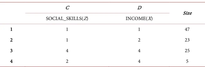
For the one hundred elderly people, build the decision table D-Table(X) shown in Table 4.

Dividing the domain with the condition collection C we get the equivalent class X =

{

[

U U1, 2

]

,

[ ] [ ]

U3 ,U4

}

, dividing the domain with the decision attribute D we get the equivalent class Y=

{

[ ] [ ]

U1 ,U2 ,

[

U U3, 4

]

}

, thus we get the follow-ing rules, accordfollow-ing to the formula 4 and 5. We can also get the reliability u(x,y) and coverage degree c(x,y). The result of rules and their equivalent classes, relia-bility and coverage is shown in Table 5.

[image:12.595.211.539.492.599.2]

Let α = 0.6 and β = 0.2, the rule R2 and R4 will be deleted. Finally we get rule R1 and R3. We can see that although R2 has larger coverage degree, but it can lead to decision confliction. Though rule R4 has higher reliability, it is the rarely ap-peared rule, it may not be true. So rule R2 and R4 should be deleted.

Table 4.D-Table(X).

C D

Size SOCIAL_SKILLS(Z) INCOME(X)

1 1 1 47

2 1 2 23

3 4 4 25

4 2 4 5

Table 5. Rule table R.

[image:12.595.206.541.636.725.2]

(13)

4. Optimization of the Evaluation Model

This section describes the optimization process for the elderly evaluation model. There four steps to perform the optimization.

1) Build the decision table based on the correlation degree of evaluation items: In turn, take one item as the decision attribute and the others as the condition attributes to build the decision table. Firstly, optimize the condition attribute in the decision table by calculating the correlation degree between each condition attribute and the decision attribute and delete the attribute that its correlation degree less than the threshold. Secondly, delete the equivalent condition attribute in the decision table. Calculate the correlation degree between each condition with all the others and delete the condition attributes whose correlation degree with this particular condition attribute is large than the degree with the decision attribute.

2) Generate the decision rules with the reliability and coverage degree.

Calculate the reliability and coverage degree for each decision equivalent class in the decision table and delete those classes whose degree is less than the thre-shold. In this way the classes that may generate the rarely appeared rules and the uncertain rules will be deleted. Then the decision rules will be created by each decision equivalent class.

3) Sort the evaluation items with the coverage degree. Use the rule merge al-gorithm to merge the rules according to the coverage degree and create the evaluation sequence of items by sorting their coverage degree in descending or-der.

4) Verify the model with accuracy and reduction rate. Use the merged rules and evaluation sequence to simulate the elderly person’s evaluation process. By calculating the reduction rate and accuracy one can verify the model.

4.1. The Evaluation Reduction Algorithm Based on the

Correlation Degree

The evaluation reduction algorithm is based on the formula in section 3.2. Eval-uation items reduction build the basis for decision rule generation and the sort-ing of the evaluation items.

For the elderly evaluation information system I =

(

U A V, ,

)

, set the threshold

(14)

DOI: 10.4236/ijis.2017.72003 38 International Journal of Intelligence Science The pseudo code is shown below.

Algorithm 1: Dependency based attribute reduction algorithm Input: I=(U A V, , ), threshold of SU: σ

Output: List (d-table)

1 Traverse every item in A as d

2 Set d as the decision attribute, the others in A as the condition attribute C, get decision _{table d-table}

3 Get all the d-table in I, named as List (d-table) 4 Traverse dt in List (d-table)

5 Traverse every item c in C 6 Calculate su of c and d. 7 If su < σ, delete c in C of dt 8 Traverse dt in List (d-table) 9 Traverse c in C of dt 10 Traverse other items c’ in C 11 Calculate su’ between c and c’ 12 Set the SU between c’ and d as su 13 If su’ < su, delete c’ in C of dt 14 Return List (d-table)

4.2. The Rule Generation Algorithm Based on Reliability and

Coverage Degree

The rule generation algorithm is based on reliability and coverage degree calcu-lation in section 3.3, which delete the equivalent decision class to generate accu-rate and effective decision rules.

Let the threshold of reliability be α, threshold of coverage degree be β. Tra-verse the dt in collection of decision table List (d-table) obtained with algorithm 1. Traverse each decision equivalent class ec-d row by row in dt, and calculate the reliability and coverage degree of ec-d. If the reliability less than α then there exists confliction in ec-d. If the coverage degree less than β, then there exist rarely appeared evaluation values, this ec-d should be deleted from dt.

Followed, traverse the ec-d in dt and generate rule set R. For each decision equivalent class ec-d, generate a set of rules in accordance with the permutation and combination of the conditional attribute set R:

{

Xi − >Yj

}

. In order to

im-prove the matching rate and to reduce the number of conditional attribute of the rules, for R generated form the same decision equivalence class, we select the rules with less condition attributes and have no conflict with rules generated from other ec-ds.

(15)

DOI: 10.4236/ijis.2017.72003 39 International Journal of Intelligence Science Algorithm 2: Credibility and coverage based rule extraction algorithm

Input: List (d-table), threshold of credibility: α, threshold of coverage: β Output: List (rule)

1 Traverse every item in List (d-table) as dt 2 Traverse every equivalence class in dt as ec-d 3 Calculate the credibility of ec-d, named as u 4 Calculate the coverage of ec-d, named as c 5 If u <α or c < β, remove ec-d from dt 6 Traverse every item in List (d-table) as dt 7 Traverse every equivalence class in dt as ec-d

8 Generate a series of rules R in every possible combination of condition attributes of ec-d 9 Traverse every item in R as r

10 If r doesn’t conflict with other rules and r has the less number of condition attributes, _{remove the rules with the more number of condition attributes from the same ec-d}

11 Return the final R, List (rule)

4.3. Evaluation Items Sort Algorithm Based on the Coverage

Degree

This part proposes the sort algorithm that can get an optimized evaluation se-quence.

If the items in antecedent of the rules have been evaluated, the items in con-sequent of the rules can be predicted by rules, so that the number of items that need to be evaluated is reduced. Therefore, in the process of evaluation, the items are ordered by their frequency in antecedent of the rules and rules’ cover-age degree.

The pseudo code is shown as follows.

Algorithm 3: Coverage based rule merging algorithm Input: List (rule)

Output: Sequence (item)

1 Traverse every item in List (rule) as r

2 Merge each item i in antecedent in List (rules) with the summation of their coverage c 3 Store m < i, c > in M

4 Sort M in descending order of the values 5 Return the keys in M as Sequence (item)

4.4. The Index for the Effective of the Method

There are two intuitive measure indexes for this elderly evaluation model. One is the reduction rate (rr) and the other is the accuracy rate of prediction (ar).

( )

len S rr

len S ′

(16)

( )

len S ar

len S ′′ =

′ (11)

where S is set of the key value pair <i, v>, i indicate i-th evaluation item and v is its value. S′ is set of the key value pair <i, v>, i indicate i-th evaluation item

and v is its predicted value. S′′ is the S′ whose prediction is correct. The

function len represents the length of the set.

The reduction rate in formula 6 reflects the effect of our method. The greater reduction rate means more obvious in the optimization of the model and the higher efficiency of the evaluation process. The accuracy of prediction in formu-la 7 reflects the quality of our method. The higher the accuracy means the pre-diction is closer to the real value. Because the real value of the evaluation items in nature is imprecise, it is very difficult get the accuracy over 95%. A good model optimization should keep 80% of accuracy and over 30% of reduction rate.

Next we simulate the elderly evaluation process and calculate the reduction rate and the accuracy. For an elderly person u, let’s evaluate his items with the evaluation Sequence (item) got from algorithm 3. For i-th item, get its value v and put it into the evaluation sequence S with the key value pair s < i, v>, in this way we can simulate the real evaluation process. With the algorithm 2 one can get the decision rule set List (rule). We will match every rule antecedents in List (rule) with the items in S. If it matches the rule than its consequent will be the predicted evaluation value and hence be added into the prediction sequence S′,

which is to predict the reduced evaluation items. Finally calculate rr with S′

and S. And calculate ar by compare with the real case evaluation data and the prediction data.

Algorithm 4 illustrates the calculation process of the two indexes.

Algorithm 4: Reduction rate and accuracy rate based model verification algorithm Input: Sequence (item), List (rule), U: List (u)

Output: reduction_rate, accuracy_rate 1 Traverse every item in List (u) as u 2 Traverse every item in Sequence (item) as i 3 Get the value v of i from u and store s < i, v> in S 4 Traverse every item in List (rule) as r

5 If S matches the antecedent of r successfully, store s < i, v> in S and S’ 6 Traverse every item in Sequence (item) as i

7 If i is not in the key collection of S, get the value v of i from u and store s < i, v> in S 8 Traverse every item in S’ as s

9 If the value v of i is equal to the value v’ of i in u, set counter to be counter+1 10 Set rr as the result of the length of S divides by the length of S’

(17)

5. Experiments

5.1. Experiment Data

Experiments are based on the actual data from Lime Family Limited Company (Lime Family for short). Lime Family has deployed dozens of elderly service sta-tion in Beijing, Yantai and Haikou three cities in China and carried out profes-sional nursing assistant training. In order to fully grasp the situation of the el-derly, the existing evaluation questionnaire in Lime Family with a total of 56 items is drafted based on the Barthel Index and the national industry standard of ability assessment for older adults. Average evaluation time for an elder person is about 15 - 20 minutes. Because there are too many items, the time is always too long to assess user dissatisfaction, so that it is urgent to propose an effective method to optimize it. The method proposed in this paper is verified in the real application background.

1) Experiment data

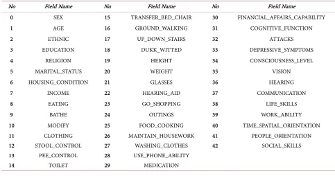
After data preprocessing, 43 items and 136 elderly evaluation data were se-lected. The total evaluation items are shown as Table 6.

2) Distribution of evaluation items’ value

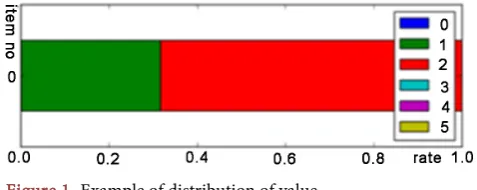
Distribution of evaluation items’ value is shown by bar graph such as Figure 1.

Figure 1 shows the value distribution of No.0 item SEX with different colors to distinguish the different values and the sum of the proportion is 100%. As

[image:17.595.54.538.477.731.2]

Figure 1 shows, there are two possible values in item SEX and value 1 is male (green) accounted for about 32% while value 2 is female (red) accounted for about 67%.

Table 6. Data information.

No Field Name No Field Name No Field Name

0 SEX 15 TRANSFER_BED_CHAIR 30 FINANCIAL_AFFAIRS_CAPABILITY

1 AGE 16 GROUND_WALKING 31 COGNITIVE_FUNCTION

2 ETHNIC 17 UP_DOWN_STAIRS 32 ATTACKS

3 EDUCATION 18 DUKK_WITTED 33 DEPRESSIVE_SYMPTOMS

4 RELIGION 19 HEIGHT 34 CONSCIOUSNESS_LEVEL

5 MARITAL_STATUS 20 WEIGHT 35 VISION

6 HOUSING_CONDITION 21 GLASSES 36 HEARING

7 INCOME 22 HEARING_AID 37 COMMUNICATION

8 EATING 23 GO_SHOPPING 38 LIFE_SKILLS

9 BATHE 24 OUTINGS 39 WORK_ABILITY

10 MODIFY 25 FOOD_COOKING 40 TIME_SPATIAL_ORIENTATION 11 CLOTHING 26 MAINTAIN_HOUSEWORK 41 PEOPLE_ORIENTATION 12 STOOL_CONTROL 27 WASHING_CLOTHES 42 SOCIAL_SKILLS 13 PEE_CONTROL 28 USE_PHONE_ABILITY

(18)

[image:18.595.252.491.73.168.2]

Figure 1. Example of distribution of value.

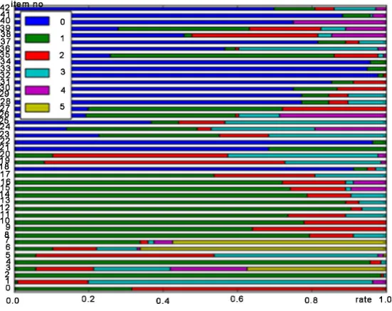
The distribution of total evaluation items’ value is shown as Figure 2. As Fig-ure 2 shows, the actual evaluation results are very unevenly distributed in vari-ous items. Different items have different number of values, which is at least 2 and up to 5. Besides, in one item, the difference among the numbers of the el-derly each value contained is relatively large with the maximum gap reached 99.24%. For example, in the data of evaluation item ATTACKS about 136 elderly people, there are 133 elderlies whose value is 0 while one person is 2 and two persons are 1.

5.2. Experiment Result

Using the methods proposed in Section 4, the correlation degree of evaluation items is calculated, and the decision rules are generated. The evaluation items are prioritized and finally the reduced and prioritized evaluation model is got. Applying the optimized evaluation model we re-evaluate the elderly and com-pare the result with the actual data to verify the effectiveness of the method. The experiment result is shown as follows.

1) Calculating the correlation degree of evaluation items

Based on the Formula 3, the correlation degree of 43 evaluation items between each other are calculated and the result is shown as Figure 3.

The horizontal and vertical axes of Figure 3 represent the identifier of evalua-tion items. The correlaevalua-tion degree result is range interval [0, 1] with the color temperature to represent the degree as value 0 indicates no correlation and value 1 indicates the strongest correlation.

By setting the threshold of SU σ = 0.2, filter out the correlation degree of evaluation items whose value is lower than σ. The result is shown as Figure 4(a). For example, after the threshold filtration, there is only 1 item that is correlated with item No.0.

(19)

[image:19.595.235.511.71.290.2]

[image:19.595.278.479.317.485.2]

Figure 2. Distribution of evaluation items’ value.

Figure 3. the correlation degree of 43 evaluation items.

(a) (b)

Figure 4. the correlation degree of 43 evaluation items.

[image:19.595.219.540.515.663.2]

(20)

DOI: 10.4236/ijis.2017.72003 44 International Journal of Intelligence Science 2) Generating the decision rules

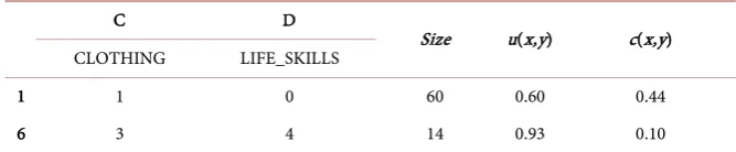
After evaluation item reduction, respectively take each item as decision attribute and receive a total of 43 decision table. Table 7 shows the decision table of No.38 item, D-Table (LIFE_SKILLS), where decision attributes D is item LIFE_SKILLS, condition attributes C is item CLOTHING, and size is the num-ber of elderlies who have the same values of condition attributes and decision attribute. Base on the Formula 3 and 4, calculate the reliability u(x,y) and cover-age degree c(x,y) of each decision equivalent class in decision table D-Table (LIFE_SKILLS).

By setting the threshold of the reliability α = 0.55 and coverage degree β = 0.1, based on algorithm 2, filter each decision equivalent class from decision table D-TABLE(LIFE_SKILLS), and the result is shown as Table 8.

Setting CLOTHING as a, and LIFE_SKILLES as d, generate the decision rules are shown in Table 9.

After applying Algorithm 2 to 4 decision tables optimized by Algorithm 1, there are a total of 61 decision rules.

3) Prioritizing evaluation items

Applying Algorithm 3 based on the 61 decision rules, we get the reduction evaluation items and the order of them. There is a total of 23 evaluation items after reduction shown as Table 10 whose identifier represents the order of eval-uation.

4) Process of optimizing evaluation

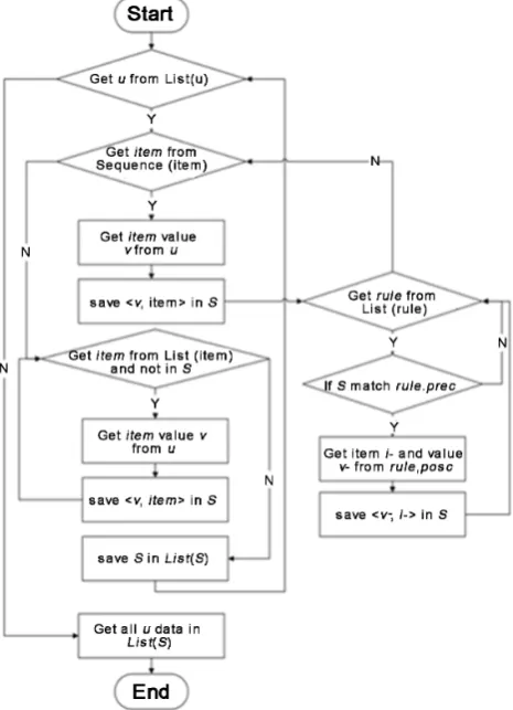
Let the 61 decision rules generated by Algorithm 2 be rule set List <rule>, the ordered evaluation items be Sequence (item), the collection of elderly evaluation result U be List (u) and all evaluation items A be List (item). The process of re-evaluation for the elderlies using the optimized evaluation model is shown in

[image:20.595.198.540.506.740.2]

Figure 5.

Table 7.D-Table (LIFE_SKILLS).

C D

Size u(x,y) c(x,y) CLOTHING LIFE_SKILLS

(21)

[image:21.595.205.539.89.158.2]

Table 8. D-Table (LIFE_SKILLS) after reduction.

C D

Size u(x,y) c(x,y) CLOTHING LIFE_SKILLS

1 1 0 60 0.60 0.44

[image:21.595.206.539.191.248.2]

6 3 4 14 0.93 0.10

Table 9. Result of decision rules.

No Generated rules u(x,y) c(x,y)

1 (a,1) −> (d,0) 0.60 0.44 2 (a,3) −> (d,4) 0.93 0.10

Table 10. Result of items-order.

No Field Name No Field Name No Field Name 1 USE_PHOME_ABILITY 9 TOILET 17 HEARING

2 LIFE_SKILLS 10 COGNITIVE_ _FUNCTION 18 CLOTHING

3 FINANCIAL_AFFAIRS_ _CAPABILITY 11 MEDICATION 19 _CONDITIONHOUSING_

4 DEPRESSIVE_SYMPTOMS 12 HEIGHT 20 INCOME

5 WORK_ABILITY 13 _ORIENTATIONPEOPLE_ 21 OUTINGS

6 ETHNIC 14 WASHING_CLOTHES 22 UP_DOWN_STAIRS

7 ATTACKS 15 TRANSFER_BED_ _CHAIR 23 GO_SHOPPING

8 STOOL_CONTROL 16 WEIGHT

First, evaluate item No.1 as the order of prioritized evaluation items. Then, according to the value of evaluated items and the decision rules, if there are some items can be inferred, infer the values of them, otherwise evaluate the next unknown item as the order of prioritized evaluation items, and so on. Finally, if all the 23 prioritized items have been evaluated and there still are some items have not the value; these not valued items can be evaluated in any order.

5) Verification the effectiveness of the method

Applying the optimized evaluation model we re-evaluate the 136 elderly. In the process, record the number of actual evaluation items compared with the number of total evaluation items, record the values of inferred items according to the decision rules compared with truth value of them, and calculate the reduc-tion rate rr and accuracy rate ar based on Formula 6 and 7.

[image:21.595.209.540.283.482.2]

(22)

[image:22.595.256.489.77.399.2]

Figure 5. Process of optimizing evaluation.

Figure 6. Line chart of RR and AR.

[image:22.595.253.491.438.625.2]

(23)

DOI: 10.4236/ijis.2017.72003 47 International Journal of Intelligence Science rate and accuracy rate respectively are 0.22 and 0.14, indicating the volatility of them is small. Generally, the optimized method proposed in this paper is effective.

5.3. Parameter Designs Analysis

In the optimized evaluation model, the threshold of SU σ, reliability α and cov-erage degree β these three parameters have an important influence on the result. In order to analyze the influence on the reduction rate and accuracy rate by these parameters, we designed the following three experiment groups so that to find the better setting of parameters.

1) Experiment group 1

Supposing the threshold of the reliability α = 0.10 and the threshold of the coverage degree β = 0.10, let the value of the threshold of the correlation degree σ increase by 0.1 from 0 to 1, which designed 11 experiments. In each experi-ment, we build decision tables, generated decision rules, carried out the evalua-tion for elderly and calculated the reducevalua-tion rate and the accuracy rate to optim-ize the model as Section 4.

Supposing the threshold of the correlation degree σ = 0.10 and the threshold of the coverage degree β = 0.10, let the value of the threshold of the reliability α increase by 0.1 from 0 to 1, which designed 11 experiments. In each experiment, we build decision tables, generated decision rules, carried out the evaluation for elderly and calculated the reduction rate and the accuracy rate to optimize the model as Section 4.

Supposing the threshold of the reliability α = 0.10 and the threshold of the correlation degree σ = 0.10, let the value of the threshold of the coverage degree β increase by 0.1 from 0 to 1, which designed 11 experiments. In each experi-ment, we build decision tables, generated decision rules, carried out the evalua-tion for elderly and calculated the reducevalua-tion rate and the accuracy rate to optim-ize the model as Section 4.

Specific parameters of these three experiment groups are shown as in Table 11.

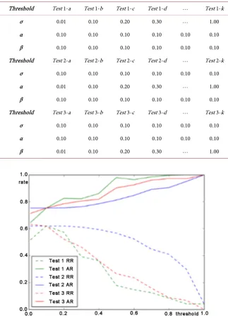
With the value of the mutative parameter in three groups as the horizontal axis and the percentage as the vertical axis, the line chart of reduction rates (RR, dotted line) and accuracy rates (AR, solid line) about three experiment groups is shown as Figure 7, which is respectively distinguished by green, blue and red.

As Figure 7 shows, there is a strong negative correlation between the reduc-tion rate and the accuracy rate. When the reducreduc-tion rate is high, the accuracy rate is always low, which is coincident with the actual situation. In the process of optimizing model, we hope both of them as high as possible. To this end, it is necessary to find the most optimal solution. In order to measure the optimality of these two indexes, we introduce the statistical method F-test.

2 RR AR

F

RR AR

× = ×

(24)

[image:24.595.212.536.87.539.2]

Table 11. Specific parameters of experiment groups.

Threshold Test 1-a Test 1-b Test 1-c Test 1-d _ Test 1-k

σ 0.01 0.10 0.20 0.30  1.00 α 0.10 0.10 0.10 0.10 0.10 0.10 β 0.10 0.10 0.10 0.10 0.10 0.10 Threshold Test 2-a Test 2-b Test 2-c Test 2-d  Test 2-k

σ 0.10 0.10 0.10 0.10 0.10 0.10 α 0.01 0.10 0.20 0.30  1.00 β 0.10 0.10 0.10 0.10 0.10 0.10 Threshold Test 3-a Test 3-b Test 3-c Test 3-d _ Test 3-k

σ 0.10 0.10 0.10 0.10 0.10 0.10 α 0.10 0.10 0.10 0.10 0.10 0.10 β 0.01 0.10 0.20 0.30  1.00

Figure 7.RR and AR line chart of experiment groups.

With the value of the mutative parameter in three groups as the horizontal axis and the F value as the vertical axis, the line chart of F values about three ex-periment groups is shown as Figure 8.

(25)

[image:25.595.239.502.74.284.2]

Figure 8.F values of experiment groups.

5.4. Comparative Experiment Analysis

In order to verify the effectiveness of the method, we designed a decision tree based experiment and expert knowledge based experiment compared with the method proposed in this paper.

1) Exp.1 decision tree based optimization experiment

First, based on C4.5 Algorithm, build 43 decision trees with the 43 evaluation items respectively as decision attribute and evaluate the No.0 items as the order of Table 6. Then, according to the value of evaluated items and the decision trees, if there are some items can be inferred, infer the values of them, otherwise evaluate the next unknown item as the order of Table 6, and so on. Finally, if all the 43 items have been evaluated, calculate the reduction rate and the accuracy rate of each elderly based on Formula 6 and 7. The experiment result is shown as

Figure 9.

As Figure 9 shows, the average of reduction rate is 34.97% and the average of accuracy rate is 61.21%, which indicates the decision tree method is not suitable for practical use because of the lower accuracy rate.

2) Exp.2 expert knowledge based optimization experiment

We set up 32 decision rules and the order of evaluation items using the know-ledge of expert in Lime Family. As the evaluation process in Section 5.2 - 4, eva-luate the 136 elderly people and the experiment result is shown as Figure 10.

As Figure 10 shows, the average of reduction rate is 14.93% and the average of accuracy rate is 85.95%. There are many of elderly people whose accuracy rate is 100%, which indicates the expert knowledge based optimization method is more considerable. However, the reduction rate is not good enough; the prob-lem of redundancy evaluation still exists.

3) Comparison results

(26)

[image:26.595.244.503.63.501.2]

[image:26.595.245.497.74.272.2]

Figure 9. RR and AR line chart of Exp.1.

Figure 10. RR and AR line chart of Exp.2.

Exp.1, expert knowledge based optimization experiment Exp.2 and experiment with method proposed in this paper Exp.3, is shown as Figure 11, which is re-spectively distinguished by green, red and blue.

As Figure 11 shows, the RR of Exp.3 is far higher than Exp.1 and Exp.2, which indicates using the method proposed in this paper to optimize the evalua-tion process will make the evaluaevalua-tion time greatly reduced and the problem of redundancy evaluation largely eliminated. Although the AR of Exp.3 is lower than Exp.2, the distribution of AR in Exp.3 is more stable than Exp.2. Moreover, the polarization between high value and low value in Exp.2 is more serious and there are some elderly people whose accuracy rate is 0.

[image:26.595.244.499.295.500.2]

(27)

[image:27.595.60.536.67.265.2]

DOI: 10.4236/ijis.2017.72003 51 International Journal of Intelligence Science (a) (b)

Figure 11.RR and AR of Exp.1, Exp.2 and Exp.3.

Table 12. indexes of three experiments.

No rr DC (rr) ar DC (ar) F

Exp.1 34.97% 0.15 61.21% 0.38 0.43 Exp.2 14.93% 0.31 85.95% 0.26 0.25 Exp.3 57.23% 0.22 82.42% 0.14 0.67

As Table 12 shows, the rr of Exp.3 is higher than Exp.1 and Exp.2 while the rr stability of Exp.3 is between others; the ar stability of Exp.3 is higher than Exp.1 and Exp.2 while the ar is between others. Generally, the F value of Exp.3 is much higher than Exp.1 and Exp.2.

6. Conclusions

This paper proposes a method for optimize the elderly evaluation model with the rough set theory. The method proposed in this paper is tested in the Lime Family Company. Real-life result shows that the method can reduce more than 40% items with over 90% accuracy prediction rate. Compared with commonly used methods in industry, our method has good performance on both reduction rate and accuracy. For example, compared with decision tree, our method has the same reduction rate performance and 20% improvement on average in ac-curacy. Compared with expert knowledge based methods, our method has the same accuracy performance and can reduce more than 30% items of evaluation. Our method helps to promote the efficiency of the evaluation process.

Future work includes analyzing the impact of parameter settings on the evalu-ation results, investigating the different importance among items, and validating with data from more companies.

Acknowledgements

[image:27.595.207.539.321.383.2]

(28)

Devel-DOI: 10.4236/ijis.2017.72003 52 International Journal of Intelligence Science opment Program (“863” Program) of China under Grant No.2015AA016009, the National Natural Science Foundation of China under Grant No.61232005. The authors wish to thank Lei Yang from Lime Family Company, who provides us the evaluation data for 200 elderly persons.

References

[1] Mahoney, F.I. and Barthel, D. (1965) Functional Evaluation: The Barthel Index. Maryland State Medical Journal, 14, 56-61.

[2] MZ/T 039-2013 (2014) Ability Assessment for Elder Adults. Standards Press of China, Beijing.

[3] Prieto, L., Alonso, J. and Lamarca, R. (2003) Classical Test Theory versus Rasch Analysis for Quality of Life Questionnaire Reduction. Health & Quality of Life Outcomes, 1, 1035-1039.

[4] Fernandez, E. and Boyle, G.J. (2001) Affective and Evaluative Descriptors of Pain in the McGill Pain Questionnaire: Reduction and Reorganization. Journal of Pain Official Journal of the American Pain Society, 2, 318-325.

https://doi.org/10.1054/jpai.2001.xbcorr25530

[5] Gurlitz, M. (2015) Forecasting SPEAK Test Score from TOEFL Score: A Bayesian Model for Screening International Teaching Assistants. Systems & Information En-gineering Design Symposium, Charlottesville, VA, 24 April 2015, 188-193.

https://doi.org/10.1109/SIEDS.2015.7116971

[6] Panigrahi, S.S. and Mantri, J.K. (2015) Epsilon-SVR and Decision Tree for Stock Market Forecasting. International Conference on Green Computing & Internet of Things. Greater Noida, Delhi, 8-10 October 2015, 761-766.

https://doi.org/10.1109/ICGCIoT.2015.7380565

[7] Liu, C. and Jiang, Q. (2009) Mixed Financial Forecasting Index System Construct and Financial Forecasting Study on the C4.5 Decision Tree. International Confe-rence on Management & Service Science, Wuhan, 16-18 September, 1-4.

https://doi.org/10.1109/ICMSS.2009.5302147

[8] Anh, L.T.N., Dau, H.X. and Phuong, N.H. (2015) Cholera Forecast Based on Asso-ciation Rule Mining. IEEE 2015 International Conference on Communications, Management and Telecommunications (ComManTel), DaNang, Vietnam, 28-30 December 2015, 133-137. https://doi.org/10.1109/ComManTel.2015.7394274

[9] Feng, H., Chen, Y., Ni, Q. and Huang, J. (2014) A New Rough Set Based Classifica-tion Rule GeneraClassifica-tion Algorithm (RGI). International Conference on Computational Science & Computational Intelligence, Las Vegas, 10-13 March 2014, 380-385. [10] Chen, Y., Qiujianlin, Chen jianping, Chen, L. and Pan, Y. (2012) A Parallel Rough

Set Attribute Reduction Algorithm Based on Attribute Frequency. International Conference on Fuzzy Systems & Knowledge Discovery, Chongqing, 29-31 May 2012, 211-215. https://doi.org/10.1109/FSKD.2012.6233881

[11] Sakai, H., Wu, M. and Yamaguchi, N. (2014) On the Definability of a Set and Rough Set-Based Rule Generation. International Conference on Advanced Applied Infor-matics, Kita-Kyushu, 31 August-4 September 2014, 122-125.

https://doi.org/10.1109/IIAI-AAI.2014.34

[12] Liu, Z. and Li, Y. (2009) A New Heuristic Algorithm of Rules Generation Based on Rough Sets. International Seminar on Business & Information Management, 1, 291-294.

(29)

DOI: 10.4236/ijis.2017.72003 53 International Journal of Intelligence Science Sciences, 11, 341-356. https://doi.org/10.1007/BF01001956

[14] Pawlak, Z., Grzymala-Busse, J., Slowinski, R. and Ziarko, W. (1995) Rough Set. Communications of the ACM, 38, 800-805. https://doi.org/10.1145/219717.219791

[15] Hu, Q., Zhang, L., An, S., Zhang, D. and Yu, D. (2012) On Robust Fuzzy Rough Set Models. IEEE Transactions on Fuzzy Systems, 20, 636-651.

https://doi.org/10.1109/TFUZZ.2011.2181180

[16] Chen, H., Li, T., Ruan, D., Lin, J. and Hu, C. (2013) A Rough-Set-Based Incremental Approach for Updating Approximations under Dynamic Maintenance Environ-ments. IEEE Transactions on Knowledge & Data Engineering, 25, 274-284.

https://doi.org/10.1109/TKDE.2011.220

[17] Liang, J., Wang, F., Dang, C. and Qian, Y. (2014) A Group Incremental Approach to Feature Selection Applying Rough Set Technique. IEEE Transactions on Knowledge & Data Engineering, 26, 294-308. https://doi.org/10.1109/TKDE.2012.146

[18] Huang, H.H. and Kuo, Y.H. (2011) Cross-Lingual Document Representation and Semantic Similarity Measure: A Fuzzy Set and Rough Set Based Approach. IEEE Transactions on Fuzzy Systems, 18, 1098-1111.

https://doi.org/10.1109/TFUZZ.2010.2065811

[19] Maji, P. and Garai, P. (2013) Fuzzy-Rough Simultaneous Attribute Selection and Feature Extraction Algorithm. IEEE Transactions on Cybernetics, 43, 1166-1177.

https://doi.org/10.1109/TSMCB.2012.2225832

[20] Albanese, A., Pal, S.K. and Petrosino, A. (2014) Rough Sets, Kernel Set, and Spati-otemporal Outlier Detection. IEEE Transactions on Knowledge & Data Engineer-ing, 26, 194-207. https://doi.org/10.1109/TKDE.2012.234

[21] Gersho, A. and Gray, R.M. (2003) Codecell Convexity in Optimal Entropy-Constrained Vector Quantization. IEEE Transactions on Information Theory, 49, 1821-1828.

https://doi.org/10.1109/TIT.2003.813478

[22] Zhu, W. and Wang, F. (2007) On Three Types of Covering-Based Rough Sets. IEEE Transactions on Knowledge & Data Engineering, 19, 1131-1144.

https://doi.org/10.1109/TKDE.2007.1044

Submit or recommend next manuscript to SCIRP and we will provide best service for you:

Accepting pre-submission inquiries through Email, Facebook, LinkedIn, Twitter, etc. A wide selection of journals (inclusive of 9 subjects, more than 200 journals)

Providing 24-hour high-quality service User-friendly online submission system Fair and swift peer-review system

Efficient typesetting and proofreading procedure

Display of the result of downloads and visits, as well as the number of cited articles Maximum dissemination of your research work

Submit your manuscript at: http://papersubmission.scirp.org/