Munich Personal RePEc Archive
Loan Refusal, Household Income and
Savings in Ghana
Koomson, Isaac and Annim, Samuel Kobina and Peprah,
James Atta
University of Cape Coast
20 August 2014
1
Loan Refusal, Household Income and Savings in Ghana
Isaac Koomson1 Samuel K. Annim
James A. Peprah
Department of Economics Faculty of Social Sciences
College of Humanities and Legal Studies University of Cape Coast
Ghana
Abstract
Loan refusal has been a problem facing many loan applicants at the household level and this problem is not new to loan applicants in Ghana. Despite this knowledge, researchers passively discuss loan refusal and do not consider the intensity of this problem. This study analyses the effect of household income and savings on loan refusal and the intensity of loan refusal in Ghana using the fifth round of the Ghana Living Standards Survey (GLSS-5). The study employs the direct elicitation approach to identifying credit constrained (loan refused) households and makes use of the Logit and Poisson regression to regress the loan refusal variable on other covariates. The Logit model is applied to loan refusal as a binary variable (refused and not refused) while the Poisson is applied to loan refusal as a count variable (number of times of loan refusal). The econometric analysis of 1,600 and 1,591 households for the loan refusal and intensity of loan refusal respectively shows that income and savings inversely relate to loan refusal and the intensity of loan refusal at their respective significance levels. It is also shown that low-income and low-savings households are more likely to be discouraged from loan applications than their counterparts in high-income and savings households. Financial institutions are called upon to generally widen their coverage and to extend their activities more into the rural areas so as to increase the stock of loanable funds available to rural dwellers. This will reduce the vulnerability of rural dwellers when it comes to loan refusal.
JEL Classification: D1, D14, D82, G21, O16
Keywords: Loan Refusal, Credit Rationing, Discouraged Borrowers, Income, Savings
2 Introduction
All over the world, it has been established that better access to credit reduces household consumption volatility, improves investment/production opportunities, eases the constraints on small and family businesses, and diversifies household and financial sector assets (IMF, 2006). The welfare gains from such expansion can be sizable, making further growth of household credit desirable. According to, Diagne, Zeller and Sharma (2000) there are, at least, two channels through which access to credit affects household welfare outcomes.
In the first instance, it alleviates the capital constraints on households. These households incur expenditure on agricultural inputs during the planting and growth periods of crops, while earnings are received several months after the harvest. The second channel is by increasing its risk-bearing ability and altering its risk-coping strategy. When a household possesses the knowledge that it can still access credit to smoothen consumption even in a situation of an income shortfall resulting from a potentially profitable but risky investment turning out to be unprofitable, that household will be prompted to bear the additional risk (Diagne et al., 2000) and may therefore be willing to adopt new, more risky technologies (Eswaran & Kotwal, 1990). Even if a household is not borrowing, the mere access to credit, with a borrowing option, helps that household to avoid adopting risk-reducing, but inefficient economic activities such as precautionary motives that come with negative returns.
However, access to credit has been a problem to households and to small businesses all over the world. Crook and Hochguertel (2005) explored credit demand and credit constraints in the U.S., Italy and the Netherlands and found that lower age and less wealth (low income) increase loan applicants’ risk of being constrained. Faced with these constraints, good borrowers who end up becoming discouraged borrowers, may not apply to banks for loans because they feel they will be rejected if they do. The feeling alone is the underlying reason for their discouragement. Of those who applied, Crook and Hochguertel went on to show that a much higher proportion is rejected in the U.S. compared to other countries. A comparative consideration of discouraged borrowers showed that a considerably small percentage of Italian and Dutch households are credit constrained, compared with U.S. households.
In Africa, Kedir, Ibrahim and Torres (2007) undertook a study in Ethiopia and found that
the two major reasons for discouragement in borrowing are households’ perception of the
success probability of their loan application and lack of collateral. For instance, 47.9 percent of the discouraged prospective borrowers did not apply because they believed they would not be successful, while 32.8 percent of them did not apply because they did not have collateral. The interest rate and loan processing time were also mentioned as deterrents to loan application. As established by Levenson and Willard (2000) and Freel et al. (2012), discouraged borrowers were recognized to be twice as many as applicants who have been denied or refused credit. Again, being constrained may vary across some demographic characteristics of borrowers (Vos, Yeh, Carter & Tagg, 2007).
In Ghana, about 90 percent of households and small firms are refused loans when they apply to the formal financial intermediaries due to inability to fulfill conditions such as collateral security (Bigsten et al., 2003). Many small firms for reasons such as very difficult processes and fear that they will be refused if even applied, do refuse to apply for formal loans. It is therefore a common phenomenon to see most of the households and small scale enterprises (SSEs) resorting
3
sources including “Susu” revolving fund and inheritance (Abor, 2007). Grundling and Kaseke (2010) showed in the FinScope Ghana 2010 report that the proportion of the adult population in Ghana who are financially served are 56 percent. From this figure, those served by the formal financial institution are 40.7 percent, those served by the informal financial institutions are 15.3 percent and those who do not have or use any financial product are 44.9 percent.
Household income also has the potential to affect a particular household’s access to credit, especially when it comes to loan refusal. According to Fernando (2007), low
income-households’ problems in accessing credit have different dimensions. The most conspicuous
dimension is that the majority of the low-income populations in developing countries do not have access to very basic financial services. In the developing economies again, it is shown that adults in the richest quintile are, on average, more than twice likely to own formal account than those in the poorest quintile (Demirguc-Kunt & Klapper, 2012). In Ghana, it has been observed that low-income people have been offered very little to no services by the formal financial sector and has, in effect, created a high demand for credit and savings services amongst the poor (Gyemibi, Mensah, Opoku, Appiah & Akyaa, 2011). From the evidence above, it is suggestive that low income households stand a higher chance of being refused loan compared to high income households.
When considering household savings, research has shown that some financial institutions place a very high premium on savings when advancing loans to potential and/or existing clients. Even in some cases, potential loan beneficiaries are required to have a pre-determined amount of savings before benefiting from any loan facility. This is what has come to be known in the literature as compulsory savings. In relation to the type of savings, Goldstein et al. (1999) in Mensah (2009) identified two categories – voluntary and compulsory savings.
4
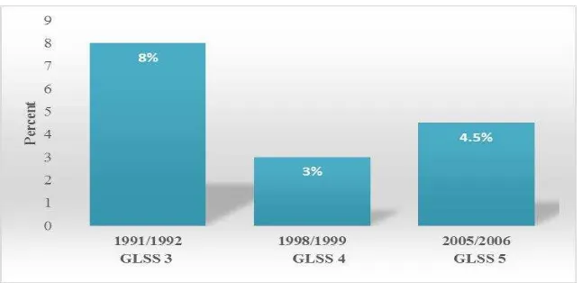
Figure 1: Percentage of Households Loan Refusals in Ghana Source: Computed from GLSS 3, GLSS 4, GLSS 5
Credit constraint facing households has several implications, ranging from child labour to
challenges in households’ consumption smoothing. Research has shown that credit constraint to
households play a role in explaining child labour (Beegle, Dehejia & Gatti, 2003), fuel domestic violence (Peprah & Koomson, 2014) and drive the use of credit for consumption, thereby making credit constraints an important impediment to inter-temporal consumption smoothing for many households (Annim, Dasmani & Armah, 2011). Loan refusal, as an extreme form of credit constraint, results in self-financing and maximizes the risk of premature liquidation of productive
investments that arise due to households’ unpredictable future liquidity crises coupled with the
slow cycle of returns. In this wise, economic agents who experience unexpected liquidity pressures may be forced to prematurely liquidate their investments in the absence of financial intermediaries, especially if they are self-financed (Bencivenga & Smith, 1991).
To explore the issue of loan refusal, Stiglitz and Weiss (1981) wrote on “Credit
Rationing in Markets with Imperfect Information” and indicated that credit constraint or loan refusal is a long-term equilibrium because of the information asymmetry and adverse selection effect. This triggered a lot of research interest as to what really causes loan refusal. Kon and Storey (2003) later developed the theory of discouraged borrowers and showed that borrowers do not apply for loans because the imperfect credit screening mechanism by financial institutions gives biased signal to borrowers into wrongly feeling that they will be rejected if they ever applied.
Jappelli (1990) and Cheng (2009) did similar studies and found income, wealth, savings and many others to be the factors that constrain access to credit. In as much as these studies give insightful revelations regarding the factors that constrain access to credit (and passively rope in loan refusal), none of them has gone a step further to examine loan refusal as the main subject of study and to even go ahead to consider the intensity (incidence) of the loan refusal. Again, a parametric study of how these variables affect loan refusal in Ghana has not been done.
5
intensity of loan refusal; and savings does not have an effect on the intensity of loan refusal. Conclusions drawn from these tests will aid in the designing of policies to reduce the problem of loan refusal to households.
Attempting to alleviate the problems associated with loan refusal will need an in-depth knowledge of what causes it. The distinct methodological approach adopted for this study will add to the very scanty literature on issues concerning loan refusal around the world and in Ghana to be specific. The concept of loan refusal has a two-pronged approach. It is either looked at from the demand-side or from the supply-side. This research is restricted to the demand-side (specifically from the household level) to look at household level characteristics that effect loan refusal which, by implication, shrouds the effects that the interplay of supply-side and household variables have on loan refusal. The remaining sections of this paper are arranged as follows: the next section covers literature, both theoretical and empirical. Section three considers the methodology which also covers data and the empirical model. Section four provides the results and discussion of findings and section six concludes the study.
Literature
The literature review begins with the theory of credit rationing, moves on to the theory of discouraged borrowers and end with the empirical literature. This sequence is chosen because the theory of discouraged borrowers, which is the main theory for this study, is quite recent and falls under the theory of credit rationing.
Afonso and Aubyn (1998) define credit rationing as a situation where demand for loans exceeds supply at the prevailing interest rate and also where the price of a loan (the interest rate) does not fully adjust to completely satisfy the demand. This means that, among loan applicants, some will get loan while others will not. Keeton (1979) explains credit rationing as occurring in two ways: either borrowers are not given the full amount of credit they applied for (“type I
rationing”) or some of them are completely turned down (“type II rationing”). The credit rationing model developed by Stiglitz and Weiss (1981) essentially stated that the interest rate that is used as a sorting device by the lender may affect the riskiness of the pool of borrowers. Stiglitz and Weiss went on to say that although the risk of a project is reflected by the variance of returns, lenders can observe the mean returns from the projects but not their variance. In the Stiglitz-Weiss model, all projects have the same mean but different variances (mean-preserving spreads). Under this sort of imperfect information, Stiglitz and Weiss show that expected returns to the lender increase with the interest rate only up to a point.
Theory of Discouraged Borrowers
6
empirical papers on credit rationing in many countries, examples of which include Berger and Udell (1992); Peterson and Rajan (1994).
Under a range of assumptions, Kon and Storey (2003) stated that the scale of discouragement in an economy depends upon the screening error of the banks, the scale of application costs and the degree to which the bank interest rate differs from that charged by the money lender. They showed that discouragement is at a maximum where there is some, but not perfect information. It can also be shown that household income also affects borrower discouragement. A study by Weller (2009) showed that the share of low-income families who felt discouraged from applying for credit was more than twice that of middle-income families and almost nine times that of high-income families. Also, interest charged on debt tend to be higher for lower-income families.
According to the study by Boucher, Carter and Guirkinger (2008) and Kon and Storey (2003) cited in Cheng (2009), two reasons account for demand-side credit constraints. One is high transaction cost and risk cost and the other is the mistakes in screening for effective borrowers and cognitive biases for the screening mechanism. Cheng (2009) went ahead to state that demand-side credit constraints could be eventually attributed to the imperfect institutional
arrangement of formal finance, but its formation is deeply related to households’ cognitive
biases and risk aversion preference. Cheng’s version of the theory of discouraged borrowers, which he specifically made demand-side, depicted the rationing of credit as occurring in three forms. These forms of credit rationing and their causes are summarized in Table 1.
Table 1: Types of Credit Rationing and their Cause Type of Credit Rationing Cause of Credit Rationing
Type I Application cost resulting preparation of application material, travelling time and cost, psychological discomfort and gifts or treating
Type II Extra cost caused by financial institutions’ inability to
effectively screen borrowers’ credit and risk
Type III Households’ risk aversion toward loan application Source: Cheng (2009)
Empirical Literature
This section reviews literature on the relationship between household level characteristics and the dependent variables used for the analysis. Although, in some cases, these variables explain their effect only from the demand, as is the focus of the paper, Kedir, Ibrahim and Torres (2007), stated that it is important to note that these variables can reflect both determinants of demand for credit and determinants of supply of credit. Hence, in some cases the effects of the independent variables on the probability of being credit constrained may be a priori ambiguous, as demand and supply factors may be working in the same direction. An example is when using educational level as an explanatory variable. While the financial institutions may place much
premium on loan applicants’ educational level and refuse granting loan to those with low
7 Household Income
Low-income households find it difficult to acquire collateral to use in securing loans. Low-income families have multiple reasons for which they would want to smoothen their income over short-term fluctuations due to less stable employment and earnings. As a result, they have an ongoing need for financial services that can make it easier for them to save or to access credit. Low-income families often lack access to financial services that middle-income families take for granted. There are a number of reasons why low-income families tend to be unbanked (United Nations, 2000). Financial institutions frequently require credit checks to open an account, set high minimum account balances, and have high overdraft-fee characteristics that are ill-suited to low-income earners (Blank & Barr, 2009). It can be inferred that household income is very vital in loan acquisition and that low-income households are more likely to be refused loans, compared to high-income households.
Savings and Loan Refusal
Some microfinance institutions (MFIs) require borrowers to make compulsory deposits before they can benefit from a loan; usually, borrowers must maintain these deposits during the life of the loan (Rosenberg, Gonzalez & Narain, 2010). About one-third of the sustainable MFIs reporting to Microfinance Information Exchange (MIX) for 2006 required such savings deposits and, on the average, these MFIs are smaller than the ones that do not use compulsory savings. Personal savings serve as a form of economic security for the household. It also provides formal financial institutions with a financial history on which they can base lending decisions (Morris & Meyer, 1993). Mohamed (2003) notes that few rural people actually make use of banks for saving and borrowing.
Adjei, Arun, and Hossain (2009) studied the Sinapi Aba Trust (SAT) and found a positive relationship between loan amount and savings deposits. Thus, all members of SAT who had benefited from loan facilities from the programme must have at least 10 per cent of such loan amount in the form of savings deposits prior to the disbursement of their loans. Such Sollateral Savings are used as guarantee for individual, and, sometimes group loans. The required sum can be as much as 50 percent of the credit one wishes to apply for.
Age of Household Head
Kimuyu and Omiti (2000) conducted an extensive study in Kenya and came out with findings which demonstrated that age is associated with access to credit in that younger applicants are likely to be refused credit than older applicants. Lore (2007) cited in Mukiri (2011) also reveals that younger loan applicants in Kenya are more likely to face constraints in accessing bank loans than older people and went ahead to state that age is an indicator of useful experience in self-selection in the credit market. This self-selection is an important aspect of decision making styles. Older applicants also tend to have higher levels of work experience, education, wealth and social contacts. These resources are important in developing key competencies. Therefore, superior age leads to higher levels of entrepreneurial orientation.
Educational Level
Again, Owuor (2009) observed in Kenya that literacy and education level have a
8
which can also limit access to credit and eventually increase the potential of possible loan refusal. Education, which translated into human capital development, is positively associated with some knowledge of bank loan application procedure (Storey, 1994). Higher levels of formal education are mostly restricted to non-poor households hardly found in the rural areas. It is therefore expected that the majority of rural households would be highly discouraged from applying for credit (Sebu, 2013).
Sex
The sex of the household head may affect the household’s probability of being refused
loan. There is a general belief that women are discriminated against informal credit markets (Mohamed, 2003). According to Amu (2005), women lack access to and/or are likely to be refused credit. In some cases, women are unwilling to access such facilities where they are available. Amu goes on to say that since banks require collateral, women who do not have land titles to use as collateral are left out of the credit market since their produce are not a good guarantee for bankers, unlike the cash crops such as cocoa, which is largely grown by men. However, Kedir et al. (2007) observed from studies in Ethiopia that formal financial institutions offered more loans to female-headed households than male-headed households.
Location
Geographic location affects a household’s access to credit. This is to say that differences
exist in rural and urban dwellers’ access to credit (Leyshon & Thrift, 1996) and that rural dwellers are discriminated against when accessing credit from financial institutions. The writers go on to say that this discrimination is mostly prominent in deprived areas such as the rural communities in Africa where there is a lack of economic and infrastructural development such as financial institutions. To them, poor locations are expected to be deprived of financial services and households that are sited in such locations may even lack the means to afford the collateral requirements. Finally, the expectation of Leyshon and Thrift was that households in the rural north and south of Malawi will be more discouraged from borrowing.
Study methodology Theoretical Model
9
Modified Version of Jappelli’s Model to suit Loan Refusal A household is not liquidity constrained if;
C* YA
1r(1) A household is said to be constrained if
C*YA
1r D(2) Where *
C is optimal consumption in the absence of the current borrowing constraint and
r
is the exogenous real rate of interest. A = the resources available to each household (non-human wealth) and D = the amount that the household can borrow. Two factors determine whether the constraint binds: (i) how much the individual would like to borrow, that is, the difference between C* and available resources; and (ii) how much financial intermediaries are willing to lend to that individual, that is, the right hand side of (2).To make the case of loan refusal operational, these three assumptions are made.
Assumptions
1. Upon application, the household either obtains the full amount or is refused entirely.
2. In the cross section the reduced form for C* is expressed as C* X'e
, where X is a matrix of observable cross-sectional variables such as current income, savings, age, demographic characteristics, education, and so on. The matrix of observables may also include quadratic and interaction terms for some variables. The vector of parameter,, is common to all households, and the vector, e, is an error term that is specific to each household. C* is further assumed to be increasing in both wealth and current income with propensities to consume out of income and savings.
3. The debt ceiling Dis also a function of the same variables as desired consumption plus an error term that captures unobservable variables, D X' . Since collaterals protect lenders from the risk of default and help them to discriminate against risky borrowers, it is assumed that D is increasing in household’s savings and current income.
After applying for the loan, equation (2) becomes, C*YA
1r D(3)
From the assumptions above, it follows that equation (3) can be rewritten as X'YA
1r
X' e 0 (4)Although desired consumption and the debt ceiling are both unobservable, the section above has identified some individuals on whom the loan refusal binds (that is, the refused applicants and the discouraged borrowers). We can then define the dummy variable as stated in equation (5), where LR represents loan refusal.
LR X' 0 (5)
0 '
if
1
X
LR (the household is refused the loan)
0 '
if
0
X
LR (the consumer is not refused the loan)
Where is a linear combination of the parameters of the expression in (2) and
e . The probability that a household is refused loan, conditional on the variables
10 Estimation Techniques and Models
Estimation of the Logit Model
(6) 1
ln 12 i
i i i i X P P L
To estimate (6), we need, apart from Xi, the values of the regressand, or logit, Li. This
depends on the type of data available for analysis. We distinguish two types of data: (1) data at the individual, or micro, level, and (2) grouped or replicated data. This study uses data at the individual/household/micro level in which case OLS estimation of (6) is infeasible. Pi = 1 if a household is refused loan and Pi = 0 if it is not refused loan. Putting these values directly into the logit Li, we obtain:
0 1 ln i
L if a household is refused loan
1 0 ln i
L if a household is not refused loan
Empirical Model Specification
(8) Re ) | 1 Pr( 8 6 6 5 4 3 2 1 0 i i i e gion b Loc b Dep b Yrsch b Age b Sex b lsave b linc b b X LR
The Poisson Regression Model – Intensity of Loan Refusal
According to Gujarati (2004), a Poisson regression treats the number of loan refusals as a Poisson random variable with an intensity hypothesized to depend on posited explanatory variables. The key assumption that underlies the Poisson Regression Model is the equality in the expected value and the variance of the error terms.
We can recall that a random variable X is Poisson distributed if its probability distribution function is given by
! Y x f y Y y
(9)Where Y 0,1,2,3,... denotes the intensity of the Poisson process and 0
While the Poisson process has been used in a variety of applications, what is emphasized in this study is its applicability in modelling loan refusal. is interpreted as the, we assume
) , (
i v . Where v a vector of explanatory variables and refusal rate. To emphasize the dependency of this refusal rate on various explanatory variables’ vector of parameters to be estimated.If the number of actual loan refusals is LRi, then according to the Poisson specification,
we have:
! exp i u LR i LR LR i i (10)
log-11
likelihood function is the logarithm of the product of the marginal probabilities.
Empirical Model for Intensity of Loan Refusal
[image:12.612.85.478.163.349.2](24) Re ) | ( 8 6 6 5 4 3 2 1 0 i i i i e gion Loc Dep Yrsch Age Sex lsave linc X LR E
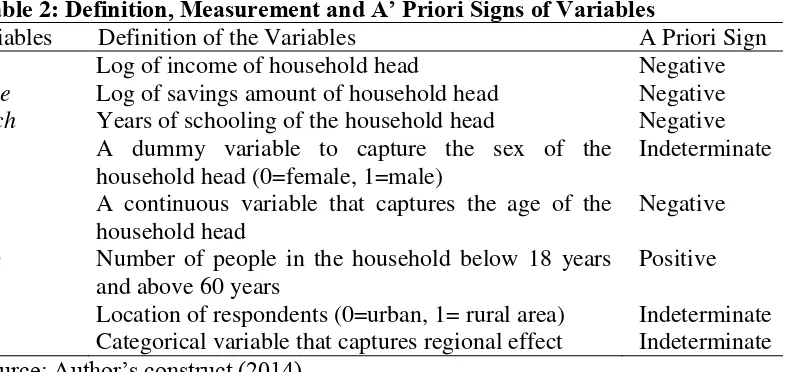
Table 2: Definition, Measurement and A’ Priori Signs of Variables
Variables Definition of the Variables A Priori Sign
linc Log of income of household head Negative
lsave Log of savings amount of household head Negative
Yrsch Years of schooling of the household head Negative Sex A dummy variable to capture the sex of the
household head (0=female, 1=male)
Indeterminate
Age A continuous variable that captures the age of the household head
Negative
Dep Number of people in the household below 18 years and above 60 years
Positive
Loc Location of respondents (0=urban, 1= rural area) Indeterminate Reg Categorical variable that captures regional effect Indeterminate
Source: Author’s construct (2014)
Data and Description
The data used for this study was sourced from the fifth round of the Ghana Living Standard Survey (GLSS-5). This data is collected by the Ghana Statistical Service (GSS) through a nation-wide survey which focuses on the household as a key socio-economic unit and provides key insights into living conditions in the country. The most recent GLSS data available was collected in 2005/2006 and contains data on household-level socio-economic characteristics such as education, health, consumption, income, economic activities and demographic characteristics as well as community information. The data gives a nationally representative sample on 8,687 households that were selected by giving each of them a non-zero probability of being selected. Data was collected by asking households to answer a set of questions and that made the study follow the direct elicitation approach to identifying credit constrained (loan refused) households
Data justification
12 Source: Derived from GLSS 5, 2005/2006
Results and Discussion Descriptive statistics
[image:13.612.87.492.79.303.2]Table 3 shows the percentage of Ghanaian households that have been refused loans. Currently, the national figure for loan refusal in Ghana stands at 4.5 percent and is greater in the rural areas (5.42%) than in the urban areas (3.43%). This means that the probability of one being refused loan in the rural area is greater than another person in the urban area. This could be attributed to the fact that loan applicants in the urban areas, on the average, lack viable businesses and are unable to write good business plans that have better potentials of securing the required capital for the realization of investment projects.
Table 3: Loan Refusal by Location in Ghana
Location
Loan Refusal
Not Refused (%) Refused (%) Total
Urban 96.57 3.43 100
Rural 94.58 5.42 100
Total 95.50 4.50 100
N= 1,600 Pearson chi2(1) = 15.5867 Pr = 0.000 Source: Computed from GLSS 5, 2005/2006
Table 4 displays the number of times (intensity) of loan refusal faced by households in Ghana. It can be seen that majority (95.2%) of the households have not suffered loan refusal, 3.2 percent of the households have suffered loan refusal once, 1.0 percent have suffered twice, 0.4 percent have suffered loan refusal thrice and 0.2 percent of the households have suffered loan Figure 2: Data justification
Total number of households=8,622
Total Missing=6,628
Final Sample Size=1,600
Household savings =1,994
Missing for Household savings =6, 628
Missing for Loan refusal = 0.00
[image:13.612.88.460.512.620.2]13
[image:14.612.79.467.119.233.2]refusal four times. It can be concluded that the highest loan refusals to been suffered by households is four, with the minimum being zero (none).
Table 4: Number of Times (Intensity) of Loan Refusal
Number of Loan Refusals Frequency Percentage
No Refusal (0) 1,523 95.2
Refused Once (1) 51 3.2
Refused Twice (2) 16 1.0
Refused Thrice (3) 6 0.4
Refused Four Times (4) 4 0.2
Totals 1,600 100
Source: Computed from GLSS 5, 2005/2006
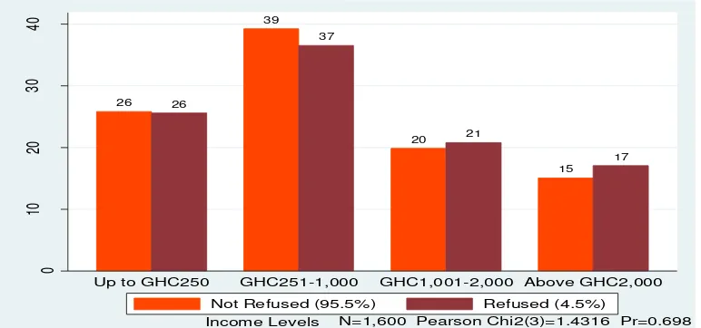
Figure 3 indicates that in spite of the initial increases in the value of both income levels and loan refusal (positive relationship), these variables began having a negative relationship beyond the initial situation. This negative relationship between income and loan refusal characterized all subsequent income categories. It should also be noted that the insignificant chi-square value can be attributed to the fact that the income categories were generated during the data management process and the boundaries were not of equal size due to challenges in the distribution of observations in the income variable. The significance of the income variable will be determined using the regression analysis, where the variable is used in the continuous form and not in categories. The inverse relationship between income and loan refusal can be seen, possibly, as emanating from the credit worthiness of high income earners since they are believed to have higher abilities of paying back the loan plus interest (BoG, 2007).
26 26
39 37
20 21
15 17
0
10
20
30
40
Up to GHC250 GHC251-1,000 GHC1,001-2,000 Above GHC2,000
Not Refused (95.5%) Refused (4.5%)
[image:14.612.76.462.434.615.2]N=1,600 Pearson Chi2(3)=1.4316 Pr=0.698 Income Levels
14
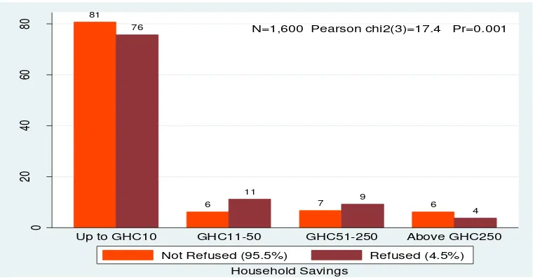
Figure 4 depicts a negative/inverse relationship between savings and loan refusal. This is because households’ savings serve as a security to the financial institutions in case of loan default. In the microfinance industry, where some microfinance institutions demand compulsory savings before granting loans, savings plays a vital role in the institutions’ loan decisions. The inverse relationship between household savings and loan refusal is not surprising because savings has always been a means by which potential borrowers prove how credit-worthy they are (Goldstein et al., 1999).
81 76
6 11
7 9 6
4
0
20
40
60
80
Up to GHC10 GHC11-50 GHC51-250 Above GHC250 Not Refused (95.5%) Refused (4.5%)
N=1,600 Pearson chi2(3)=17.4 Pr=0.001
[image:15.612.76.456.195.395.2]Household Savings
Figure 4: Loan Refusal by Savings Categories Source: Computed from GLSS 5, 2005/2006
15
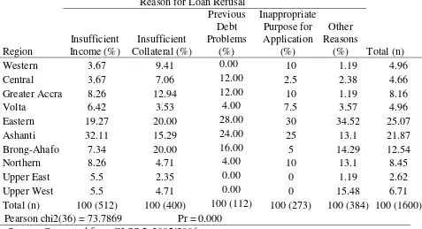
Table 5: Reasons for Loan Refusal by Administrative Regions (Across-Group Frequencies)
Reason for Loan Refusal
Region
Insufficient Income (%)
Insufficient Collateral (%)
Previous Debt Problems
(%)
Inappropriate Purpose for Application
(%)
Other Reasons
(%) Total (n)
Western 3.67 9.41 0.00 10 1.19 4.96
Central 3.67 7.06 12.00 2.5 2.38 4.66
Greater Accra 8.26 12.94 12.00 10 1.19 8.16
Volta 6.42 3.53 4.00 7.5 3.57 4.96
Eastern 19.27 20.00 28.00 30 34.52 25.07
Ashanti 32.11 15.29 24.00 25 13.1 21.87
Brong-Ahafo 7.34 20.00 16.00 5 14.29 12.54
Northern 8.26 4.71 4.00 10 13.1 8.45
Upper East 5.5 2.35 0.00 0 1.19 2.62
Upper West 5.5 4.71 0.00 0 15.48 6.71
Total (n) 100 (512) 100 (400) 100 (112) 100 (273) 100 (384) 100 (1600) Pearson chi2(36) = 73.7869 Pr = 0.000
Source: Computed from GLSS 5, 2005/2006
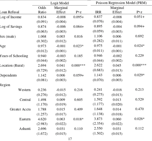
Regression results
Regression Analysis on the Effect of Income and Savings on Loan Refusal
The study focuses on two main variables, income and savings, and how they influence the likelihood of loan refusal. These results have been presented in Table 5. The Pseudo R2 =
0.1222 indicates that 12 percent of the variations in loan refusal is explained by the covariates. Post-estimation tests like the linktest and Hosmer-Lemeshow were conducted to test for model specification and goodness-of-fit respectively. The scores for _hat (P>|z|= 0.041) and _hatsq (P>|z|=0.797) for the linktest shows that the model is correctly specified. This means that we can, only by chance, find additional predictors that are statistically significant. As regards the goodness-of-fit test, the Hosmer-Lemeshow gave a score of Prob > chi2 = 0.4566 which is greater than 0.05 and indicates that the model is of good-fit. In this model, the savings variable has a near perfect relationship with the Upper East and Upper West regional dummies and they are dropped for consistency in coefficients.
Household income has a negative relationship with loan refusal. This indicates that a
GH₵1.00 increase in household income reduces the likelihood of being refused loan (compared
16
On household savings, this study finds an inverse relationship between this variable and loan refusal. It can be seen from the regression analysis that holding all other variables constant, a GH₵1.00 increase in savings amount decreases the likelihood of a household being refused loan, compared to not being refused, by a factor of 0.838 at a 10 percent significance level. It can
be inferred that savings, in the Ghanaian context, plays an integral role in a household’s access to
credit. Thus, not having enough savings amount increases the likelihood of a household being refused loan upon application. Goldstein et al. (1999), cited in Mensah (2009), showed how beneficiaries are required to possess a certain quantum of savings before benefiting from any loan facility. Low-savings households, by implication, will also have a higher perception of being turned down and, in effect, be discouraged from applying for loans (Cheng, 2009).
Age of the household head also inversely relates to loan refusal and can be attributed to the fact that as people age, their acquisition of more social and economic resources places them at a vantage point when it comes to loan acquisition and reduces their probability of being refused loans. Regarding the location of a loan applicant (in this case, rural area), the regression analysis shows that a loan applicant in the rural area stands a higher risk of being refused, compared to another applicant in the urban area. This could stem from the limited number of financial institutions in the rural areas which also limits the total amount of loanable funds available thereby increasing the tendency of financial institutions to resort to rationing and discouraging of
borrowers. Finally, the number of dependents is positively related to loan refusal. An increase in
the number of dependents by one person increases the likelihood of being refused loan, compared to not being refused, by a factor of 1.142 at an alpha level of 10 percent, holding all other variables constant. This relationship can be deduced as arising from the huge pressure on the income of the household used for consumption purposes and which leaves them with very little income to fall on in times of need.
Regression Analysis on the Effects of Income and Savings on the Intensity of Loan Refusal This section puts forward the findings from the Poisson regression model (PRM) (from Table 5) which considers, into detail, the earlier discussed binary loan refusal variable to now look at the binary variable as a count variable, taking into account the number of times of loan refusals beyond one. This is what has been considered as the intensity of loan refusal. Just like the logit model, the exponential of the Poisson regression coefficient gives the incidence rate ratio (IRR) and is used in the analysis that follows.
Household income is inversely related to the intensity of loan refusal. A GH₵1.00
increase in household income decreases the likelihood of the intensity of loan refusal by a factor 0.837 at 10 percent alpha level, holding all other variables constant. This seeks to explain that low income households stand a higher risk of being intensely refused. This finding is supported by that of McKenchnie (2005) who was of the view that the intensity of loan refusal for low-income households is likely to be more because they lack the collateral needed to secure financial transactions. Low-income households’ lack of collateral also leads them to be cognitively biased into thinking that they will be refused if they apply for loan. This eventually turn low-income households into discouraged borrowers (Weller, 2007).
Going on to household savings, it can be seen that the intensity of loan refusal is likely to
be reduced by a factor of 0.895 as a result of a GH₵1.00 increase in the amount of household
17
MFIs require borrowers to make before they can benefit from a loan. Low savings also turn households into discouraged borrowers because they feel they stand a higher risk of being refused (Cheng, 2009).
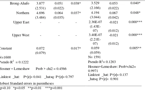
[image:18.612.79.572.261.718.2]The age of the household head also inversely relates to the intensity of loan refusal in that as the household head ages, the likelihood of the rate ratio of refusal decreases by a factor of 0.975 at a significance level of five percent, holding all other variables constant. It can be deduced that younger household heads stand a greater risk of being discouraged from loan application (Kon & Storey, 2013) and so do rural dwellers (Leyshon & Thrift, 1996). Regarding location, it can be deduced from Table 6 that residing in the rural area is likely to increase the intensity of loan refusal by a factor of 2.622 more than residing in the urban area at a 0.1 percent alpha level, holding all other variables constant. Finally, an increase in the number of dependents in a household increases the intensity of loan refusal by a factor of 1.143 as the number of dependents in household increase.
Table 6: Logit Model for Loan Refusal
Logit Model Poisson Regression Model (PRM)
Loan Refusal
Odds Ratio
Marginal
Effect P>z IRR
Marginal
Effect P>z
Log of Income 0.834 -0.008 0.095+ 0.837 -0.008 0.051+
(0.091) (0.004) (0.076) (0.004)
Log of Savings 0.874 -0.006 0.064+ 0.895 -0.004 0.094+
(0.063) (0.003) (0.059) (0.003)
Sex (male) 1.068 0.003 0.816 1.106 0.006 0.692
(0.302) (0.012) (0.282) (0.011)
Age 0.973 -0.001 0.023* 0.975 -0.001 0.024*
(0.012) (0.001) (0.011) (0.001)
Years of Schooling 0.940 -0.003 0.185 0.946 -0.002 0.229
(0.044) (0.002) (0.044) (0.002)
Location (Rural) 2.694 0.041 0.000*** 2.622 0.045 0.000***
(0.729) (0.012) (0.683) (0.013)
Dependents 1.142 0.006 0.059+ 1.143 0.006 0.029*
(0.081) (0.003) (0.070) (0.003)
Region
Western 0.236 -0.015 0.216 0.241 -0.016 0.213
(0.276) (0.012) (0.275) (0.013)
Central 1.498 0.009 0.605 1.592 0.013 0.529
(1.170) (0.019) (1.177) (0.020)
Greater Accra 1.788 0.015 0.409 1.648 0.014 0.470
(1.257) (0.017) (1.138) (0.018)
Eastern 4.620 0.063 0.018* 3.873 0.060 0.026*
(2.983) (0.022) (2.354) (0.022)
Ashanti 2.696 0.031 0.110 2.550 0.031 0.112
18 Table 6 Continued
Brong-Ahafo 3.877 0.051 0.038* 3.529 0.053 0.040*
(2.531) (0.022) (2.166) (0.022)
Northern 4.696 0.064 0.037* 4.194 0.067 0.048*
(3.484) (0.035) (3.044) (0.042)
Upper East - - - 2.36E-07 -0.021 0.000***
(1.43E-07) (0.012)
Upper West - - - 3.40E-07 -0.021 0.000***
(2.21E-07) (0.012)
Constant 0.072 0.017* 0.059 0.005**
(0.079) (0.059)
N=1600 N= 1591
Pseudo R2 = 0.1222 Pseudo R2= 0.1263
Hosmer – Lemeshaw Prob > chi2 = 0.4566 Hosmer–Lemeshaw: Prob>chi2= 0.9971
Linktest _hat: P>|z|= 0.041 _hatsq: P>|z|= 0.797 Linktest _hat: P>|z|= 0.137 _hatsq: P>|z|= 0.901
Robust Standard errors in parentheses + p<0.10 *p<0.05 **p<0.01 ***p<0.001
Source: Computed from GLSS 5, 2005/2006
Conclusions and policy reflections
From the analysis on household income and loan refusal, both in the logit and Poisson models, it was shown that Ghanaian households with low income are refused loans and that the formal financial institutions have provided very little or no services to low-income households which has, in turn, created a high demand for credit among the poor. With the reasons cited above, low-income households stand a greater risk of being refused loans compared to their high-income counterparts, which makes low-income households likely to be discouraged from taking loans.
On household savings, the phenomena of compulsory savings was seen as taking centre stage in the process of loan acquisition. Savings requirement is so entrenched that some institutions see these savings amounts as another avenue to secure the loan that is to be advanced. Low-savings households then perceive that they will be turned down if they are to apply for loans, which makes them discouraged borrowers.
19 References
Abor, J. (2007). Capital structure and financing of SMEs: empirical evidence from Ghana and South Africa. Stellenbosch: Stellenbosch University. Retrieved on 2/10/2013 from http://scholar.sun.ac.za/handle/10019.1/21522
Adjei, J., Arun, T., & Hossain, F. (2009). Asset building and poverty reduction in Ghana: The case of microfinance. Savings and Development, 265–291.
AFONSO, A., & AUBYN, M. S. (1998). Credit rationing and monetary transmission: evidence for Portugal, Estudos de economia. Estud. Econ.), Lisboa, 19(1), 5–19.
Amu, N. J. (2005). The role of women in Ghana’s economy. Friedrich Ebert Foundation. Retrieved from http://library.fes.de/pdf-files/bueros/ghana/02990.pdf
Annim, S. K., Dasmani, I., & Armah, M. (2011). Does Access and Use OF Financial Service Smoothen Household Food Consumption? Retrieved on 20/11/213 from http://mpra.ub .uni-muenchen.de/29278/
Beegle, K., Dehejia, R., & Gatti, R. (2003). Child labor, crop shocks, and credit constraints. National Bureau of Economic Research. Retrieved from http://www.nber.org/papers /w10088
Benati, L. (2001). Some empirical evidence on the “discouraged worker”effect. Economics Letters, 70(3), 387–395.
Bencivenga, V. R., & Smith, B. D. (1991). Financial intermediation and endogenous growth. The Review of Economic Studies, 58(2), 195–209.
Berger, A. N., & Udell, G. F. (1992). Some evidence on the empirical significance of credit rationing. < Em> Journal of Political Economy</em>, 100(5), 1047.
Bigsten, A., Collier, P., Dercon, S., Fafchamps, M., Gauthier, B., Gunning, J. W., Söderbom, M. ans. (2003). Credit constraints in manufacturing enterprises in Africa. Journal of African Economies, 12(1), 104–125.
Blank, R. M., & Barr, M. S. (2009). Insufficient funds: Savings, assets, credit, and banking among low-income households. Russell Sage Foundation.
Cheng, Y. (2009). Credit constraints under interaction of supply rationing and demand depression: evidence from rural households in China. Retrieved on 01/01/2014 from http://smartech.gatech.edu/handle/1853/36659
Crook, J., & Hochguertel, S. (2005). Household debt and credit constraints: evidence from OECD countries. Working Paper Series-University of Edinburgh Management School, 5. De Meza, D., & Webb, D. C. (1987). Too much investment: a problem of asymmetric
information. The Quarterly Journal of Economics, 102(2), 281–292.
Demirguc-Kunt, A., & Klapper, L. (2012). Measuring Financial Inclusion: The Global Findex Database. Retrieved on 18/04/2014 from https://openknowledge.worldbank.org/handle/ 10986/6042
Diagne, A., Zeller, M., & Sharma, M. (2000). Empirical measurements of households’ access to
credit and credit constraints in developing countries: Methodological issues and evidence. International Food Policy Research Institute.
Eswaran, M., & Kotwal, A. (1990). Implications of credit constraints for risk behaviour in less developed economies. Oxford Economic Papers, 42(2), 473–482.
20
http://www.microfinancegateway.org/gm/document-1.9.26149/Low-Income%20 Households%20 Access%20t.pdf
Freel, M., Carter, S., Tagg, S., & Mason, C. (2012). The latent demand for bank debt:
characterizing “discouraged borrowers.” Small Business Economics, 38(4), 399–418. Grundling, I., & Kaseke, T. (2010). FinScope Ghana 2010. Launch Presentation (FinMark
Trust).
Gujaratı, D. N. (2004). Basic econometrics. McGraw-Hill New York.
Gyemibi, K. A., Mensah, G., Opoku, C., Appiah, T., & Akyaa, A. (2011). Credit Management Practices of Micro Financial Institution (Case Study of Multi Credit Savings and Loans). Christian Service University College Department of Business Studies.
IMF. (2006). Household Credit Growth in Emerging Market Countries.
Jappelli, T. (1990). Who is credit constrained in the US economy? The Quarterly Journal of Economics, 105(1), 219–234.
Kedir, A., Ibrahim, G., & Torres, S. (2007). Household-level credit constraints in urban Ethiopia.
University of Leicester, Nottingham Trent University and Catholic University of Uruguay.
Keeton, W. R. (1979). Equilibrium credit rationing. Garland New York. Retrieved from http://www.getcited.org/pub/101893360
Kimuyu, P., & Omiti, J. (2000). Institutional impediments to access to credit by micro and small scale enterprises in Kenya (Vol. 26). Citeseer.
Kon, Y., & Storey, D. J. (2003). A theory of discouraged borrowers. Small Business Economics,
21(1), 37–49.
Levenson, A. R., & Willard, K. L. (2000). Do firms get the financing they want? Measuring credit rationing experienced by small businesses in the US. Small Business Economics,
14(2), 83–94.
Leyshon, A., & Thrift, N. (1996). Financial exclusion and the shifting boundaries of the financial system. Environment and Planning A, 28(7), 1150–1156.
Mensah, M. M. (2009). The Role and Challenges of Savings and Loans Companies in Ghana. Kwame Nkrumah University of Science and Technology. Retrieved on 11/11/2013 from http://dspace.knust.edu.gh:8080/xmlui/bitstream/handle/123456789/686/Mercy%20Muri el%20Mensah.pdf?sequence=1.
Mohamed, K. (2003). Access to formal and quasi-formal credit by smallholder farmers and artisanal fishermen: A case of Zanzibar. Mkuki na Nyota Publishers.
Morris, G. A., & Meyer, R. L. (1993). Women and financial services in developing countries: a review of the literature. Ohio State University.
Mukiri, W. G. (2011). Determinants of access to Bank credit by micro and small enterprises in Kenya. Beacon Consultant Service.
Owuor, G. (2009). Can Group Based Credit Uphold Smallholder Farmers Productivity and Reduce Poverty in Africa? Empirical Evidence from Kenya. In 111th Seminar, June 26-27, 2009, Canterbury, UK. European Association of Agricultural Economists.
Peprah, J. A. & Koomson, I. (2014). Economic Drivers of Domestic Violence among Women: A Case Study of Ghana. Globalization and Governance in the International Political Economy, 166.
21
Rosenberg, R., Gonzalez, A., & Narain, S. (2010). The new moneylenders: are the poor being exploited by high microcredit interest rates? (Vol. 92). Emerald Group Publishing Limited.
Sebu, J. (2013). Farm households’ access to credit: who needs and who gets? Evidence from
Malawi. Journal of Economic Literature.
Stiglitz, J. E., & Weiss, A. (1981). Credit rationing in markets with imperfect information. The American Economic Review, 71(3), 393–410.
Storey, D. J. (1994). Understanding the small business sector. Cengage Learning emea.
United Nations. (2000). Microfinance and Poverty Eradication: Strengthening Africa’s
Microfinance Institutions. United Nations, New York.
Vos, E., Yeh, A. J.-Y., Carter, S., & Tagg, S. (2007). The happy story of small business financing. Journal of Banking & Finance, (2648-2672), 31.