Confidence Intervals for the Mean of Non Normal Distribution: Transform or Not to Transform

http://www.scirp.org/journal/ojs ISSN Online: 2161-7198

ISSN Print: 2161-718X

Confidence Intervals for the Mean of

Non-Normal Distribution: Transform

or Not to Transform

Jolynn Pek

1

, Augustine C. M. Wong

2

, Octavia C. Y. Wong

1

1_{Department of Psychology, York University, Toronto, Canada}

2_{Department of Mathematics and Statistics, York University, Toronto, Canada}

Abstract

In many areas of applied statistics, confidence intervals for the mean of the population are of interest. Confidence intervals are typically constructed as-suming normality although non-normally distributed data are a common oc-currence in practice. Given a large enough sample size, confidence intervals for the mean can be constructed by applying the Central Limit Theorem or by the bootstrap method. Another commonly used method in practice is the back-transformation method, which takes on the following three steps. First, apply a transformation to the data such that the transformed data are nor-mally distributed. Second, obtain confidence intervals for the transformed mean in the usual manner, which assumes normality. Third, apply the back- transformation to obtain confidence intervals for the mean of the original, non-transformed distribution. The parametric Wald method and a small sample likelihood-based third order method, which can address non-normality, are also reviewed in this paper. Our simulation results suggest that common approaches such as back-transformation give erroneous and misleading re-sults even when the sample size is large. However, the likelihood-based third order method gives extremely accurate results even when the sample size is small.

Keywords

Back-Transformation, Bootstrap, Central Limit Theorem, Delta Method, Maximum Likelihood Estimate, Third Order Method

1. Introduction

In the last two decades, there has been a push in psychological science to

im-How to cite this paper: Pek, J., Wong, A.C.M. and Wong, O.C.Y. (2017) Confi-dence Intervals for the Mean of Non-Normal Distribution: Transform or Not to Trans-form. Open Journal of Statistics, 7, 405-421.

https://doi.org/10.4236/ojs.2017.73029

Received: April 17, 2017 Accepted: June 5, 2017 Published: June 8, 2017

Copyright © 2017 by authors and Scientific Research Publishing Inc. This work is licensed under the Creative Commons Attribution International License (CC BY 4.0).

prove research reporting with an emphasis on effect size and confidence interval reporting (see American Education Research Association [1]; Cumming [2]; Wilkinson and the Task Force for Statistical Inference [3]). Effect sizes commu-nicate the magnitude and direction of a practically important effect (e.g., treat-ment decreased depression scores by 13%), and confidence intervals communi-cate this effect’s estimate precision. The importance of confidence intervals, their basic construction, and interpretation have thus been the focus of several in-fluential pedagogical articles (e.g., see Cumming and Fidler [4]; Cumming and Finch [5]; Greenland et al. [6]).

Most, if not all, modern introductory statistics textbooks review and describe the construction of confidence intervals (e.g., see Moore et al. [7]). Let

(

x1,,xn

)

be a sample obtained from a normally distributed population with mean

µ

and variance σ2_{. Then a}

(

)

1−α 100% confidence interval for

µ

can be

calcu-lated by

* *

,

x x

s s

x t x t

n n

 _{− +} 

 

  (1)

where

(

)

2

2

1 _, 1 _,

1

n n

i i

i i

x

x x x

x s

n n

= =

−

= =

−

∑

∑

and t* is the

(

1−

α

2 100

)

th _{percentile of the Student} t _{distribution with}

(

)

1

n− degrees of freedom. Moreover, when the sample size n is large (usually stated n

is larger than 30), then the

(

1−α

)

100% confidence interval for

µ

can still be

obtained from (1) except that we replaced t* by z*, which is the

(

1−

α

2 100

)

th

percentile of the standard normal distribution.

The fundamental assumption underlying the construction of this confidence interval is that the data are normally distributed. However, collected data are usually non-normally distributed in practice (for examples in psychology, see Cain et al. [8]; Micceri [9]). In public health research, Bland and Altman [10] reported that serum triglyceride measurements are distributed with positive skewness. In biology, McDonald [11] reported that the number of Eastern mud- minnows in Maryland streams are non-normally distributed.

Section 4 to compare the accuracy of the methods discussed in this paper and il-lustrated that the likelihood-based third order method gives extremely accurate coverage probability even when the sample size is small, the Wald method, the Central Limit Theorem method and then bootstrap method all performed poorly when sample size is small but the performance increases when the sample size increases, and the popular back-transformation method should not be used be-cause it does not construct the confidence interval for the correct parameter. Fi-nally, some concluding remarks are given in Section 5.

2. Methodology

This section reviews four commonly used methods, namely the Central Limit Theorem, bootstrap, back-transformation, and Wald for obtaining a confidence interval for the mean of a non-normal distribution. A very accurate likelih-ood-based method is also introduced in this section.

2.1. Central Limit Theorem Method

Let

(

x1,,xn

)

be a sample from a non-normal distribution with mean

ψ

. When the sample size n is large, the Central Limit Theorem gives

( )

( )

0,1

X

var X

ψ

− _→



where 1

n i i X

X n =

=

∑

_and var X

( )

var X

( )

n

= _{. Since} x and s2x are the unbiased

estimates of

ψ

and var X

( )

respectively; by the Central Limit Theorem, an approximate

(

1−α

)

100% confidence interval for

ψ

is

* *

,

x x

s s

x z x z

n n

 _{− +} 

 

  (2)

where *

z is the

(

1−

α

2 100

)

th percentile of the standard normal distribution.

2.2. Bootstrap Method

The bootstrap method is a popular non-parametric method, which does not re-quire any distributional assumptions. Efron and Tibshirani [12] provide a de-tailed review of the bootstrap method. The following is an algorithmic approach of obtaining a

(

1−α

)

100% percentile bootstrap confidence interval for the

population mean,

ψ

. Sample:

(

x1,,xn

)

Step 1: Resample the observed sample with replacement and calculate the sample mean for this bootstrap sample.

Step 2: Repeat Step 1 B times, where, typically, B≥200.

Step 3: Sort the B bootstrapped sample means; the

(

α

2 100

)

th and

(

1−

α

2 100

)

th _{percentiles give the}

(

)

1−α 100% percentile bootstrap

confi-dence interval for the population mean.

requires the observed sample size to be large so as to be representative of the population.

2.3. Back-Transformation Method

Recall that X is a non-normally distributed random variable with mean ψ. As-sume there exists a transformation g

( )

⋅ such that Y =g X

( )

is normally dis- tributed with mean µ and variance σ2_{. By the delta method,}

( )

1

( )

1

( )

_,

E X E g Y g

ψ _{= = } − _≈ − µ

 

and an approximate

(

1−α

)

100% confidence interval for

ψ

from (1) is

1 * sy _, 1 * sy _.

g y t g y t

n n

− −

    

− +

    

 _{   }

  (3)

It is important to note that (3) could be misleading because 1

( )

g−

µ

can be very different from

ψ

. For example, if X follows a _lognormal

(

µ σ_, 2

)

distribution,

then Y =log

( )

X is distributed as

(

2

)

,

µ σ

 . It follows that the delta method gives ψ =E X

( )

≈exp

( )

µ . However, as shown in Table 1, ψ _=exp

(

µ σ₊ 2 ₂

)

,

which can be quite different from exp

( )

µ , especially when σ2 is large.

Con-sider another example where Y= X follows a _

(

µ σ_, 2

)

distribution. Here,

the delta method gives ψ µ_≈ 2_{. However, Table 1 shows that} ψ µ₌ 2₊σ2_, which can be quite different from µ2_{, especially when} σ2 _{is large.}

The rest of this subsection is to provide a systematic way of choosing the transformation g

( )

⋅ . In practice, the most common simple transformations are the logarithmic transformation and square root transformation. Box and Cox [13] proposed a more complicated transformation, which requires the determi-nation of the power parameter. Similarly, Tukey [14] suggested a ladder of pow-er transformation, which also requires the detpow-ermination of the powpow-er parametpow-er. We review Tukey’s method in a later subsection. With an observed sample

(

x1,,xn

)

, our aim is to obtain confidence intervals for

ψ

. In this paper, focus

is placed on the two most commonly used transformations in practice: the loga-rithmic transformation and the square root transformation. Note that the tans-formation methods discussed can be generalized to any known transtans-formation in theory (cf., Box-Cox or Tukey’s transformations).

[image:4.595.206.538.617.737.2]

When observed data are non-normally distributed, a common approach is to first apply a transformation such that the transformed data become somewhat

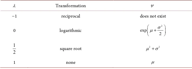
Table 1. Transformation and the parameter of interest.

λ Transformation ψ

−1 reciprocal does not exist

0 logarithmic exp 2

2

σ µ

 ₊ 

 

 

1

2 square root

2 2

µ +σ

normally distributed. In the statistical literature, two very similar families of transformations are frequently discussed: the Box-Cox transformation and Tu-key’s ladder of power transformation. In particular, Osborne [15] gives a de-tailed discussion of the application of the Box-Cox transformation. Mathemati-cally, the Box-Cox transformation and Tukey’s ladder of power transformation are very similar. Because Tukey’s ladder of power transformation is easier to in-terpret compared to the Box-Cox transformation, we review the ladder of power transformation and suggested criteria to choose an appropriate transformation to address non-normally distributed data below.

Tukey’s ladder of power transformation takes the form

( )

log if 0

if 0

X Y X

X

λ λ

λ λ

= 

= =  _≠



where

λ

is called the power parameter of this transformation, where

λ

is chosen such that Y is approximately normally distributed. Moreover,

λ

should be chosen such that the power parameter is easy to interpret. Note that

λ

=1 is

equivalent to no transformation. In practice, the popular reciprocal transforma-tion, logarithmic transformatransforma-tion, and square root transformation are equivalent to λ = −1, 0 and 1

2, respectively.

Table 1 presents the mean of distribution prior to transformation, ψ, in terms of µ and σ2 based on the type of transformation used. Since ψ does not exist for the reciprocal transformation, this transformation is not considered in this paper.

With an observed sample, we suggest the choice of

λ

be based on three criteria:

1. de-trended normal quantile-quantile (Q-Q) plot, 2. p-value of the Shapiro-Wilk test of normality, and 3. skewness.

First, when the de-trended normal Q-Q plot deviates from the horizontal ref-erence line which indicates identical quantiles between the data and a theoretical normal distribution, the plot suggests that the data are likely non-normally dis-tributed. Second, simulation studies by Razali and Wah [16] illustrate that the Shapiro-Wilk test is the most powerful test among all formulated statistical tests for normality. Under the assumption of a normal distribution, the smaller the

p-value associated with the Shaprio-Wilk test, the more evidence against the normality assumption. Thus, the transformation which gives the largest p-value of the Shapiro-Wilk test is associated with the least evidence against the trans-formed data being normally distributed. Finally, with regard to skewness, the normal distribution has skewness 0. In this vein, the transformation which re-sults in a skewness value closest to 0 is most symmetric and would be the pre-ferred transformation.

2.4. Wald Method

random variable with mean

ψ

_{and there exists a transformation} g

( )

⋅ such

that Y =g X

( )

is normally distributed with mean

µ

and variance σ2.

Moreover,

(

2

)

,

ψ ψ µ σ= _.

The log-likelihood function concerning Y can be written as

(

2

)

2

(

)

2

2 1 1 , log 2 2 n i i n a y

µ σ σ µ

σ =

= − −

∑

−

 (4)

where a is an additive constant. Without loss of generality, a is set to zero he-reafter. The overall maximum likelihood estimate (MLE), denoted by

(

2

)

ˆ ˆ,

µ σ ′_, can be obtained by solving

(

)

₍

₎

2

2

2 1 ˆ ˆ,

, ₁ ˆ 0 ˆ n i i y µ σ µ σ µ

µ σ =

∂ = − = ∂

∑



(

)

₍

₎

2 2 2

2 2 4

1 ˆ ˆ,

, ₁ ˆ 0. ˆ ˆ 2 2 n i i n y µ σ µ σ µ

σ σ σ =

∂

= − + − =

∂

∑



Hence, we have

(

) (

2

)

2

2

1

1 1

ˆ , ˆ ˆ .

n y i i n s y y n n

µ σ µ

=

−

= =

∑

− =

The observed information matrix is the negative of the second derivatives of the log-likelihood function with respect to the parameters:

(

)

(

)

(

)

(

)

2 4 1 2 2

4 4 6

1 1 1 , . 1 1 2 n i i n n i i i i n y j n y y µ σ σ µ σ µ µ

σ σ σ

= = =  ₋      =   − − + −    

∑

∑

∑

The variance-covariance matrix for

(

2

)

ˆ ˆ,

µ σ ′ can be approximated by the in-verse of Fisher’s expected information matrix,

{

_{E j}

(

µ σ_, 2

)



}

−1

  , which, in

gen-eral, can be difficult to obtain in practice. Nevertheless, the variance-covariance matrix for

(

2

)

ˆ ˆ,

µ σ ′ can be approximated by the inverse of the observed infor-mation evaluated at the MLE, _j−1

(

µ σ_{ˆ ˆ,} 2

)

where

(

)

2

2

4

0 ˆ

ˆ ˆ, .

0 ˆ 2 n j n σ µ σ σ     =        

It is well-known that

(

2

)

ˆ ˆ,

µ σ ′ _{is asymptotically distributed as normal with}

mean

(

2

)

,

µ σ ′ and variance 1

(

_{ˆ ˆ}2

)

,

j− µ σ .

Recall that the parameter of interest is ψ ψ µ σ₌

(

_, 2

)

, and we denote

(

2

)

ˆ ˆ ˆ,

ψ ψ µ σ= _{. By the delta method,}



_{( )}

(

)

(

)

(

) (

(

)

)

2 2

1 2

2 2

ˆ ˆ, ˆ ˆ, ˆ ˆ ˆ,

, ,

var

ψ

µ σ

j

µ σ

µ σ

µ σ

µ σ

(

)

(

)

(

)

(

)

( )

2

2 2

2 ₂

2 ˆ ˆ,

ˆ ˆ, ˆ ˆ,

.

, ˆ ˆ,

µ σ µ σ

µ σ _µ

µ σ _{µ σ}

σ _∂    ∂ _{ ∂ } =   ∂ _{∂ }  _∂      

Thus, an approximate

(

1−α

)

100% confidence interval for

ψ

is



_{( )}



_{( )}

(

* *

)

ˆ z var ˆ , ˆ z var ˆ .

ψ − ψ ψ+ ψ (5)

For the case of the logarithmic transformation (i.e., Tukey’s ladder of power transformation where

λ

=0), the parameter of interest is ψ =exp

( )

γ , where

2

2

γ µ σ= + _{. Therefore, by the Wald method, a}

(

1−α

)

100% confidence in-

terval for

γ

is



_{( )}



_{( )}

(

* *

)

ˆ z var ˆ ,ˆ z var ˆ

γ − γ γ + γ

where _ˆ 2

ˆ ˆ 2

γ µ σ= + and 

( )

ˆ ˆ2 ˆ4 2

var

n n

σ σ

γ ≈ + _{. Thus, an approximate}

(

1−α

)

100%

confidence interval for

ψ

is



_{( )}

{

*

}

{

* 

_{( )}

}

ˆ ˆ ˆ ˆ

exp γ z var γ , exp γ z var γ .

 _{− +} 

 

 

For the case of the square root transformation (i.e., Tukey’s (1977) ladder of power transformation where 1

2

λ= _{), the parameter of interest is} ψ µ₌ 2₊σ2_.

Therefore, an approximate

(

1−α

)

100% confidence interval for

ψ

is given by

(5), where



_{( )}

2

(

2 2

)

2 2 2ˆ 2ˆ ˆ

ˆ ˆ ˆ andvar ˆ .

n

σ µ σ

ψ µ= +σ ψ = +

2.5. Likelihood-Based Third Order Method

Both the Central Limit Theorem method and Wald method have a theoretical rate of convergence of

( )

1 2

O n− , and both the back-transformation method and

the bootstrap method have no known rate of convergence. In recent years, many methods have been developed to improve the rate of convergence of existing asymptotic methods. In this subsection, we review the modified signed log-like- lihood ratio method by Barndorff-Nielsen [17]. The modified signed log-like- lihood ratio statistic is defined as

( ) ( ) ( )

( )

( )

* * 1 _logr

r r r

r q

ψ

ψ ψ

ψ ψ

= = − (6)

where

( )

(

)

{

(

) (

)

}

1 2

2 2

ˆ 2 ˆ ˆ, ˆ ,ˆ

r ψ =sign ψ ψ− _ µ σ − µ σψ ψ _ (7) is the signed log-likelihood ratio statistic,

(

_{ˆ ,ˆ}2

)

ψ ψ

( )

q ψ is a statistic based on the log-likelihood function given in (4). Barndorff- Nielsen [17] showed that *

r is asymptotically distributed as a standard normal distribution with a rate of convergence of

(

3 2

)

O n− . Thus, a

(

1−α

)

100%

confidence interval obtained based on *

r is

(

ψ ψL, U

)

such that ψL and ψU satisfies *

( )

*

L

r ψ <z , r*

( )

ψU <z*, and ψL<ψU.

If the model is an exponential family model and the parameter of interest

ψ

is a component parameter of the canonical parameter, Fraser [18] showed that

( )

q ψ is the standardized MLE statistic. Given a general model and this idea in mind, Fraser and Reid [19] first approximate the model using an approximate tangent exponential model to obtain the locally defined canonical parameter. Then, they express the parameter of interest in terms of the locally defined ca-nonical parameter and also derived the variance the estimated parameter of in-terest in this locally defined canonical parameter scale. Thus, q

( )

ψ is the stan-dardized MLE statistic expressed in the locally defined canonical parameter scale, and the modified signed likelihood ratio statistic can be used to obtain confi-dence interval for

ψ

. Details of this algorithmic approach of obtaining *

r is outlined below.

Notation: _

( )

θ _{is the log-likelihood function;}

θ

_{is a k-dimensional vector of parameters;}

( )

ϕ ϕ θ= _{is a k-dimensional vector of canonical parameters for the} exponen-tial family model;

( )

ψ ψ θ= _{is a scalar parameter of interest;}

(

x1,,xn

)

is the observed data.

Aim: Inference about

ψ

_.

Step 1: From the log-likelihood function, obtain the overall MLE,

( ) ( )

ˆ_{, ˆ} ˆ _, ˆ

θ ψ ψ θ

= _

θ

_and ˆ_{j= jθθ}

( )

θ

ˆ _{can be obtained.}

Step 2: Apply the Lagrange multiplier technique to obtain the constrained MLE at ψ ψ= 0. More specifically, maximize

(

,

)

( )

(

( )

0

)

H θ λ = θ +λ ψ θ −ψ

with respect to

(

θ λ,

)

, where

λ

is defined as the Lagrange multiplier. Denote

the result of the maximization be

(

θ λ

 ψ0,

)

.

Step 3: Define the tilted log-likelihood function as

( )

θ =

( )

θ +λ ψ θ

(

( )

−ψ

)

 

 

where ψ is a fixed value. Obtain the constrained MLE either from the tilted log-likelihood function or from Step 2,

θ

_ψ,

( ) ( )

θ

_ψ = 

θ

_ψ and j_θθ

( )

θ

_ψ , which is the matrix of the negative of the second derivatives of the tilted log-likelihood function.

Step 4: The signed log-likelihood ratio statistic is

(

)

{

( )

( )

}

1 2

ˆ

ˆ 2 .

r=sgn ψ ψ− _ θ − θψ _ Step 5: Define

( )

( ) ( )

1

( )

= _{θ ψ θ ψ}

where ψ θθ

( )

is the first derivative of ψ θ

( )

with respect to

θ

, and ϕ θθ

( )

is the first derivative of ϕ θ

( )

_{with respect}

θ

. This quantity is a recalibration of the parameter of interest

ψ

in the canonical parameter

ϕ

space.

Step 6: The quantity

( )

ˆ

( )

ψ

χ θ

−

χ θ

 _{measures the departure of} ψˆ from

ψ

in

ϕ

space.

Step 7: The estimated variance for the departure in

ϕ

space is given by



(

( )

( )

)

( ) ( ) ( ) ( ) ( )

( ) ( )

2 1

2

ˆ _.

ˆ ˆ

j j

var

j

θ ψ θθ ψ θ ψ θθ ψ θ ψ

ψ

θθ θ

ψ θ θ ψ θ θ ϕ θ

χ θ χ θ

θ ϕ θ

− −

− ′

−  =       

Step 8: The standardized MLE departure under the

ϕ

scale is given by

(

)

( )

( )



(

( )

( )

)

ˆ

ˆ .

ˆ

q sign

var

ψ

ψ

χ θ χ θ

ψ ψ

χ θ χ θ

−

= −

− 



Step 9: The modified signed log-likelihood ratio statistic is given by

* 1

logr.

r r

r q

= −

Although the algorithm involves many steps, it can easily be implemented into algebraic or statistical software such as MATLAB, Maple and R.

3. Empirical Examples

In this section, the different methods of constructing a confidence interval about the mean of non-normally distributed data are illustrated with two empirical examples. We demonstrate that the results obtained by the methods discussed in this paper can be very different.

3.1. Example 1: Serum Triglyceride Measurements

[image:9.595.206.539.655.735.2]

Bland and Altman [10] considered n = 278 serum triglyceride measurements, which had a positively skewed data distribution with an average of 0.51 mmol/l and a standard deviation of 0.22 mmol/l. By applying a base 10 logarithm trans-formation to the data to obtain a less skewed distribution, the transformed dis-tribution became bell-shaped with an average of −0.33 and a standard deviation of 0.17. By applying the Central Limit Theorem, they report a 95% confidence interval for the mean serum triglyceride measurements to be (0.48, 0.54). Using the back-transformation method, the corresponding interval is (0.45, 0.49). Ta-ble 2 presents the 95% confidence intervals for the mean serum triglyceride

Table 2. 95% confidence interval for the mean serum triglyceride measurements.

measurements for the alternative methods reviewed above Note that for this example, the bootstrap method cannot be applied because the original data set is not unavailable.

Bland and Altman [10] noted that the interval obtained by the back-trans- formation method is actually the 95% confidence interval for the geometric mean of serum triglyceride measurements instead of the mean serum triglyce-ride measurements, where the latter is the parameter of interest. Stated diffe-rently, the back-transformation method does not provide information about the focal parameter of interest (i.e., the mean of the non-normal distribution). From Table 2, it can be observed that the results from the Central Limit Theorem me-thod are different from those obtained by the Wald meme-thod and third order method. Additionally, the Wald method and third order method give results which agree up to the second decimal place. This observation is not surprising because these two methods theoretically converge to the same answer when the sample size goes to infinity. The only difference is that the third order method will have a faster rate of convergence than the Wald method (i.e., _{O n}

( )

−1 2

versus

(

3 2

)

O n− , respectively). The different rates of convergence are more

formally illustrated in Section 4.

3.2. Example 2: Abundance of Eastern Mudminnows

McDonald [11] reported on data on the abundance of Eastern mudminnows in Maryland streams, which is reproduced below:

38 1 13 2 13 20 50 9 28 6 4 43

[image:10.595.209.541.591.734.2]

These data are non-normally distributed and McDonald [11] suggested that both the logarithmic and square root transformed data are suitable for analysis because they are more normally distributed compared to the original and other competing transformations. His final analysis makes use of the logarithmic transformed data.

Table 3 presents the 95% confidence intervals for the mean of the non-trans- formed distribution obtained by applying the Central Limit Theorem method

Table 3. 95% confidence intervals for the mean of the abundance of Eastern mud- minnows in Maryland streams.

and the bootstrap method with B = 5000 to the original data; and the back- transformation method, Wald method, and likelihood-based third order method to both the logarithmic transformed data and square root transformed data.

The results obtained by the methods discussed in this paper are very different for different transformations. In particular, the logarithmic transformation re-sults in a much larger upper bound of the interval compared to the square root transformation. Thus, it is essential to identify which transformation is more appropriate for a given set of data.

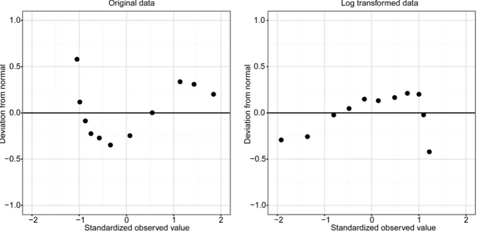
The de-trended normal Q-Q plots for the original data, logarithmic trans-formed data and square root transtrans-formed data are shown in Figure 1. From

[image:11.595.65.535.236.464.2]

these plots, it is obvious that the original data are not normally distributed be-cause the points deviate from the horizontal reference line, which indicates iden-tical quantiles between the data and a theoreiden-tical normal distribution. The two sets of transformed data are more closely normally distributed because the points in the de-trended normal Q-Q plots lie more closely to the reference line relative to the original data.

The Shapiro-Wilk test on normality of the original data gives a p-value of 0.1091. The same test on the logarithmic transformed data gives a p-value of 0.5261, and it gives a p-value of 0.6479 on the square root transformed data. Consistent with the de-trended Q-Q plot, the p-values of the Shapiro-Wilk test similarly suggest that the two transformed data sets are more likely to be nor-mally distributed. Additionally, the empirical skewness of the original data, lo-garithmic transformed data, and square root transformed data are 0.5864, −0.4886, and 0.1632, respectively. These quantifications of skewness imply that the square root transformed data are more symmetrical than the original data and logarithmic transformed data. Thus, based on the criteria discussed in Sec-tion 2.3, the square root transformaSec-tion is recommended for these data.

4. Simulation Study

A simulation study was carried out to compare the accuracies of the methods discussed in this paper. R code for the simulation is available to the interested reader upon request. For each

(

n, ,µ σ

)

combination, we generated 10,000

samples from

(

2

)

,

µ σ

 . These are our simulated transformed samples, and the non-transformed (i.e., original) samples can be obtained by applying the in-verse transformation to the simulated data. The transformations examined are the natural logarithm and square root. For each simulated sample, we computed a 95% confidence interval for the mean of the untransformed population from the five reviewed methods: Central Limit Theorem, bootstrap (B = 5000), back- transformation, Wald, and likelihood-based third order. The following quanti-ties are recorded: the proportion of true means falling within the 95% confidence interval (coverage proportion), the proportion of true means less than the lower 95% confidence limit (lower error), and the proportion of true means greater than the upper 95% confidence limit (upper error). The nominal values of cov-erage, lower error, upper error, and bias are: 0.95, 0.025, and 0.025, respectively. We present only a small subset of the simulations we conducted to highlight several key points below, and other simulation results are available upon request.

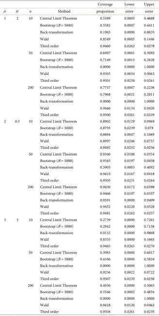
Table 4 presents results with the natural logarithmic transformed data being generated from

(

2

)

,

µ σ

 and the parameter of interest is exp 2 2

σ µ

 

+

 

 .

[image:13.595.210.539.88.737.2]

Table 4. 95% coverage probability for the logarithmic transformation case.

Coverage Lower Upper

µ σ n Method proportion error error

method give similar results. The Wald method seems to converge faster than the Central Limit Theorem and bootstrap methods. As discussed in Section 2, the back-transformation method gives unacceptable coverage probability because it is constructing confidence intervals about a parameter that is not of interest.

It can be observed that the likelihood-based third order method outperforms the other methods especially when the sample size is small; coverage, lower and upper errors associated with the likelihood-based third order method are rela-tively closer to nominal rates compared to the alternative methods. Among the remaining methods, the Central Limit Theorem method and the bootstrap me-thod give similar results. The Wald meme-thod seems to converge faster than the Central Limit Theorem and bootstrap methods. As discussed in Section 2, the back-transformation method gives unacceptable coverage probability because it is constructing confidence intervals about a parameter that is not of interest.

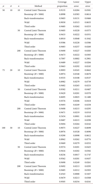
Table 5 presents results with the square root transformed data being generated from

(

2

)

,

µ σ

 and the parameter of interest is µ2₊σ2_.

Similar to results in Table 4, we can observe that the likelihood-based third order method outperforms the other methods, especially when sample size is small. In this context, the Central Limit Theorem method and the bootstrap method give similar results and they seem to converge faster than the Wald me-thod. The back-transformation method continues to give unacceptable coverage probability because it constructs confidence intervals about a parameter that is not of interest.

Based on these simulation results, the Central Limit Theorem method, boot-strap method and Wald method converge slowly relative to the likelihood-based third order method. Hence, we recommend using the likelihood-based third or-der method to obtain confidence intervals for the mean of the non-transformed distribution after applying a normalizing transformation to non-normal data, especially for small sample sizes or large departures from normality. It is impor-tant to note that researchers should not use the popular back-transformation method despite its simplicity except for the special case where ψ =E X

( )

( )

(

)

1 g− E Y

= _.

More simulations have been performed with the same pattern of results. They are not reported here, but are available upon request.

5. Conclusion

When interest is in constructing a confidence interval about a non-normal dis-tribution, normalizing transformations are typically recommended as a first step. This paper recommends the use of de-trended normal Q-Q plots, the largest

[image:15.595.209.537.90.735.2]

Table 5. 95% coverage probability for the square root transformation case.

Coverage Lower Upper

µ σ n Method proportion error error

likelihood-based third order method because of its superior performance in terms of its rate of convergence, coverage, and accuracy relative to the Central Limit Theorem, bootstrap and Wald methods, even when the sample size is small or the distribution is far from being normal.

Acknowledgements

We thank the editor and the referee for their comments. This work was based on O.C.Y. Wong’s undergraduate honors thesis. J. Pek was supported by the Natu-ral Sciences and Engineering Research Council of Canada Discovery Grant (RGPIN-04301-2014) and the Early Researcher Award by the Ontario Ministry of Research and Innovation (ER15-11-004). A.C.M. Wong was supported by the Natural Sciences and Engineering Research Council of Canada Discovery Grant (RGPIN-163597-2012).

References

[1] American Education Research Association (2006) Standards for Reporting on Em-pirical Social Science Research in AERA Publications. Educational Researcher, 35, 33-40. https://doi.org/10.3102/0013189X035006033

[2] Cumming, G. (2014) The New Statistics: Why and How. Psychological Science, 25,

7-9.https://doi.org/10.1177/0956797613504966

[3] Wilkinson, L. and the Task Force on Statistical Inference (1999) Statistical Methods in Psychology Journals: Guidelines and Explanations. American Psychologist, 54, 594-604. https://doi.org/10.1037/0003-066X.54.8.594

[4] Cumming, G. and Fidler, F. (2009) Confidence Intervals: Better Answers to Better Questions. Journal of Psychology, 217, 15-26.

https://doi.org/10.1027/0044-3409.217.1.15

[5] Cumming, G. and Finch, S. (2001) A Primer on the Understanding, Use, and Cal-culation of Confidence Intervals that Are Based on Central and Noncentral Distri-butions. Educational and Psychological Measurement, 61, 532-574.

https://doi.org/10.1177/0013164401614002

[6] Greenland, S., Senn, S.J., Rothman, K.J., Carlin, J.B., Poole, C. Goodman, S.N. and Altman, D.G. (2016) Statistical Tests, P Values, Confidence Intervals, and Power: A Guide to Misinterpretations. European Journal of Epidemiology, 31, 337-350. https://doi.org/10.1007/s10654-016-0149-3

[7] Moore, D.S., McCabe, G.P. and Craig, B.A. (2014) Introduction to the Practice of Statistics 8th Edition, W.H. Freeman and Company, New York.

[8] Cain, M.K., Zhang, Z. and Yuan, K.H. (2016) Univariate and Multivariate Skewness and Kurtosis for Measuring Nonnormality: Prevalence, Influence and Estimation. Behavior Research Methods, 1-20.

https://doi.org/10.3758/s13428-016-0814-1

[9] Micceri, T. (1989) The Unicorn, the Normal Curve and Other Improbable Crea-tures. Psychological Bulletin, 105, 156-166.

https://doi.org/10.1037/0033-2909.105.1.156

[10] Bland, J.M. and. Altman, D.G. (1996) Transformations, means, and confidence in-tervals. British Medical Journal, 312, 1079.

https://doi.org/10.1136/bmj.312.7038.1079

[12] Efron, B. and Tibshirani, R.J. (1994) An Introduction to the Bootstrap. Chapman and Hall, New York.

[13] Box, G.E. and Cox, D.R. (1964) An Analysis of Transformation (with Discussion). Journal of the Royal Statistical Society B, 26, 211-252.

[14] Tukey, J.W. (1977) Exploratory Data Analysis. Addison-Wesley, Massachusetts. [15] Osborne, J.W. (2010) Improving Your Data Transformation: Applying the Box-Cox

Transformation. Practical Assessment, Research & Evaluation, 15, Article 12. [16] Razali, N. and Wah, Y. (2011) Power Comparisons of Shapiro-Wilk,

Kolmogo-rov-Smirnov, Lilliefors and Anderson-Darling tests. Journal of Statistical Modeling and Analytics, 2, 21-33.

[17] Barndorff-Nielsen, O.E. (1991) Modified Signed Log Likelihood Ratio. Biometrika, 78, 557-561. https://doi.org/10.1093/biomet/78.3.557

[18] Fraser, D.A.S. (1991) Statistical Inference: Likelihood to Significance. Journal of American Statistical Association, 86, 258-265.

https://doi.org/10.1080/01621459.1991.10475029

[19] Fraser, D.A.S. and Reid, N. (1995) Ancillaries and Third Order Significance. Utilitas Mathematica, 7, 33-53.

Submit or recommend next manuscript to SCIRP and we will provide best service for you:

Accepting pre-submission inquiries through Email, Facebook, LinkedIn, Twitter, etc. A wide selection of journals (inclusive of 9 subjects, more than 200 journals)

Providing 24-hour high-quality service User-friendly online submission system Fair and swift peer-review system

Efficient typesetting and proofreading procedure

Display of the result of downloads and visits, as well as the number of cited articles Maximum dissemination of your research work