A constriction factor based particle swarm optimization for economic dispatch

A CONSTRICTION FACTOR BASED PARTICLE SWARM OPTIMIZATION FOR

ECONOMIC DISPATCH

Shi Yao Lim, Mohammad Montakhab, and Hassan Nouri Bristol Institute of Technology,

University of the West of England, Frenchay Campus,

Coldharbour Lane, Bristol, BS16 1QY, United Kingdom. E-mail: [email protected]

KEYWORDS

Constriction factor, economic dispatch (ED), non-smooth optimization, particle swarm optimization (PSO).

ABSTRACT

This paper presents an efficient method for solving the non-smooth economic dispatch (ED) problem with valve-point effects, by introducing a constriction factor into the original particle swarm optimization (PSO) algorithm. The proposed constriction factor based particle swarm optimization (CFBPSO) combines the original PSO algorithm with a constriction factor. The application of a constriction factor into PSO is a useful strategy to ensure convergence of the particle swarm algorithm. To verify the feasibility and performance, the proposed method is applied to a test non-smooth ED problem with valve-point effects. The results of the CFBPSO are compared with the results of other methods; the genetic algorithm (GA); the evolutionary programming (EP); the modified PSO; and in particular the improved PSO (IPSO).

1. INTRODUCTION

Under the new deregulated electricity industry, power utilities try to achieve high operating efficiency to produce cheap electricity. High operating efficiency minimizes the cost of a kilowatt-hour to a consumer and the cost to the company delivering a kilowatt-hour in the face of constantly rising prices for fuel, labor, supplies, and maintenance. Operational economics involving power generation and delivery can be subdivided into two parts. Economic dispatch (ED), as one part is called, has the distribution of generated power at lowest cost as its main objective. Minimum-loss, as the second part is called, deals with minimum-loss delivery of the generated power to the loads.

The ED of power generating units has always occupied an important position in the electric power industry. ED is a computational process where the total required generation is distributed among the generation units in operation, by minimizing the selected cost criterion, subject to load and operational constraints. For any specified load condition, ED determines the power output of each plant (and each generating unit within the plant) which will minimize the overall cost of fuel needed to serve the system load (Wood and Wollenberg 1996). ED is used in real-time energy

management power system control by most programs to allocate the total generation among the available units, unit commitment, etc. ED focuses upon coordinating the production cost at all power plants operating on the system.

In the traditional ED problem, the cost function for each generator has been approximately represented by a single quadratic function and is solved using mathematical programming based optimization techniques such as lambda-iteration method, gradient-based method, etc. (Park et al. 2006). These methods require incremental fuel cost curves which are piece-wise linear and monotonically increasing to find the global optimal solution. Unfortunately, the input-output characteristics of generating units are inherently highly non-linear due to valve-point loadings. Thus, the practical ED problem with valve-point effects is represented as a non-smooth optimization problem with equality and inequality constraints. This makes the problem of finding the global optimum solution challenging. Dynamic programming (DP) method (Liang and Glover 1992) is one of the approaches to solve the non-linear and discontinuous ED problem, but it suffers from the problem of “curse of dimensionality” or local optimality. In order to overcome this problem, several alternative methods have been developed such as evolutionary programming (EP) (Yang et al. 1996), genetic algorithm (GA) (Walters and Sheble 1993), tabu search (Lin et al. 2002), neural network (Lee 1998), and particle swarm optimization (Eberhart and Shi, 2000; Shi and Eberhart, 2001).

in many areas.

Since its introduction, PSO has attracted much attention from researchers around the world. Many researchers have indicated that the PSO often converges significantly faster to the global optimum but has difficulties in premature convergence, performance and the diversity loss in optimization process. Clerc, in his study on stability and convergence of PSO has indicated that use of a constriction factor may be necessary to insure convergence of the particle swarm algorithm (Clerc 1999). His research indicated that the inclusion of properly defined constriction coefficients increases the rate of convergence; further, these coefficients can prevent explosion and induce particles to converge on local optima.

In this paper, a novel approach is proposed to the non-smooth ED problem with valve-point effects using a constriction factor based PSO (CFBPSO). The proposed CFBPSO combines the original PSO algorithm with a constriction factor. The application of a constriction factor into PSO is a useful strategy to ensure convergence of the particle swarm algorithm. Unlike other evolutionary computation methods, the proposed method ensures the convergence of the search procedure based on the mathematical theory. In order to verify the feasibility, the proposed method is tested on a three-generator power system and the results are compared with those of other methods and in particular the improved PSO (IPSO) (Park et al. 2006) in order to demonstrate its performance. The results indicate the applicability of the proposed CFBPSO method to the practical ED problem.

The rest of the paper is structured as follows. The ED problem formulation is described in Section 2. In Section 3, the proposed CFBPSO algorithm for solving the ED problem is explained. Section 4 presents the simulation results and comparison with those of other methods. Finally, in Section 5, conclusions are drawn, based on the results found from the simulation analyses in Section 4.

2. ECONOMIC DISPATCH FORMULATION A. Basic Economic Dispatch Formulation

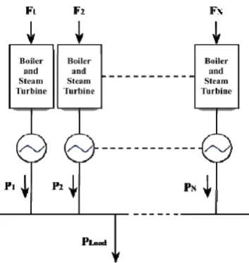
[image:2.595.341.518.61.248.2]

Fig. 1 shows the configuration that will be studied in this section. This system consists of N generating units connected to a single busbar serving a received electrical load, P_load. The input to each unit, shown as F_i represents the cost rate of the unit i. The output of each unit, P_i is the electrical power generated by that particular unit. The total cost rate of this system is the sum of costs of each of the individual units. The essential constraint on the operation of this system is that the sum of the output powers must equal the load demand. It is obvious, in the case that the generators are connected to the same busbar, the losses are zero, but if the generators are located in distant geographic locations, the losses will not be zero or close to zero. For simplicity, in this phase of the research, we assume that the losses are zero.

Fig. 1: N generating units committed to serve a load.

Mathematically speaking, the problem may be stated very concisely. That is, an objective function F_T, is equal to the total cost for supplying the indicated load. The problem is to minimize F_T subject to the operating constraints of the power system. .

The objective of the ED problem is to minimize the total cost of generation under various system and operational constraints while satisfying the power demand. The primary concern of an ED problem is the minimization of its objective function. The total cost generated that meets the demand and obeys all other constraints associated is selected as the objective function. In general, the ED problem can be formulated mathematically as a constrained optimization problem with an objective function of the form:

F_T = F_i

( )

P_i

i=1

N

∑

(1)

where F_T is the total generation cost; N is the total number of generating units; F_i is the power generation cost function of the ith unit.

Generally, the fuel cost of a thermal generation unit is considered as a second order polynomial function

F_i

( )

P_i =a_i+b_iP_i+c_iP_i2 (2)

where P_i is the power of the ith generating unit;

a_i, b_i, c_i are the cost coefficients of the ith generating unit.

This model is subjected to the following constraints.

1) Real Power Balance Equation

For power balance, an equality constraint should be satisfied. The total generated power should be the same as total load demand plus the total line loss

P_i

i=1

N

where P_Demand is the total system demand and P_Loss is the total line loss. For simplicity, transmission loss is not considered in this paper (i.e., P_Loss=0 ).

2) Unit Operating Limits

There is a limit on the amount of power which a generator can deliver. The power output of any generator should not exceed its rating nor should it be below that necessary for stable operation. Generation output of each generator should lie between maximum and minimum limits. The corresponding inequality constraints for each generator are

P_i,min≤P_i≤P_i,max (4)

where P_i is the output power of generator i; P_i,min and

P_i,max are the minimum and maximum power outputs of generator i, respectively.

B. Economic Dispatch with Valve-Point Effect

[image:3.595.43.284.352.517.2]

The generating units with multi-valve steam turbines exhibit a greater variation in the fuel-cost functions (Park et al. 2006). The valve opening process of multi-valve steam turbines produces a ripple-like effect in the heat rate curve of the generators. These “valve-points” are illustrated in Fig. 2.

Fig. 2: Incremental fuel cost versus power output for a 5 valve steam turbine unit.

Fig. 2 shows that the cost curve increases at a greater rate with power production just as a valve is opened. The reason for this is that the so-called throttling losses due to gaseous friction around the valve-edges are greatest just as the valve is opened and taper off as the valve opening increases and the steam flow smoothens.

The significance of this effect is that the actual cost curve function of a large steam plant is not continuous but more important it is non-linear. Thus, the cost function contains higher order nonlinearity. To model the effects of “valve-points”, a recurring sinusoid contribution is added to the cost function. Therefore, equation (2), the basic quadratic equation for the fuel cost of a thermal generation unit should be replaced by equation (5) to consider the valve-point effects. The valve-point effects are taken into consideration in the ED problem by superimposing the basic quadratic fuel-cost characteristics with the rectified sinusoid

component as follows:

( )

i i i i i i i

(

i

(

i i

)

)

i P a bP cP e f P P

F = + + + × × ,min −

2

sin (5)

where e_i and f_i are the coefficients of generator i reflecting valve-point effects. Note that ignoring valve-point effects, some inaccuracy would be introduced into the resulting dispatch.

3. CONSTRICTION FACTOR BASED PARTICLE SWARM OPTIMIZATION

A. Basic Concept of Particle Swarm Optimization

Particle swarm optimization (PSO) is a population based stochastic optimization technique developed by Kennedy and Eberhart in 1995, discovered through simplified social model simulation (Kennedy and Eberhart 1995). It stimulates the behaviors of bird flocking involving the scenario of a group of birds randomly looking for food in an area. All the birds don’t know where the food is located, but they just know how far they are from the food location. So, an effective strategy for the bird to find food is to follow the bird which is nearest to the food. PSO is motivated from this scenario and is developed to solve complex optimization problems.

In the conventional PSO, suppose that the target problem has n dimensions and a population of particles, which encode solutions to the problem, move in the search space in an attempt to uncover better solutions. Each particle has a position vector of X_i and a velocity vector V_i. The position vector X_i and the velocity vector V_i of the ith particle in the n-dimensional search space can be represented as

X_i=

(

x_i1, x_i2, ..., x_in

)

and V_i=

(

v_i1, v_i2, ..., v_in

)

, respectively. Each particle has a memory of the best position in the search space that it has found so far

(

Pbest_i

)

, and knows the best location found to date by all the particles in the swarm

(

Gbest

)

. Let Pbest_i=

(

x_iPbest₁ , x_iPbest₂ , ..., x_inPbest

)

and

Gbest

=

(

x

₁Gbest

,

x

₂Gbest

,

...,

x

_nGbest

)

be the best position of the individual i and all the individuals so far, respectively. At each step, the velocity of the ith particle will be updated according to the following equation in the PSO algorithm:

V_ik+1=ωV_ik+c₁r₁×⎜ _⎝ ⎛ Pbest_ik−X_ik⎞ _⎠ ⎟ +c₂r₂×⎛ _⎝ ⎜ Gbestk−X_ik⎞ _⎠ ⎟ (6)

where,

V

i k+1

velocity of individual i at iteration k+1,

V

_ik velocity of individual i at iteration k,

ω inertia weight parameter,

c₁, c₂ acceleration coefficients,

r₁, r₂ random numbers between 0 and 1,

X_ik position of individual i at iteration k,

Pbest_ik best position of individual i at iteration k,

In this velocity updating process, the acceleration coefficients c₁, c₂ and the inertia weight ω are predefined and r₁, r₂ are uniformly generated random numbers in the range of [0, 1]. In general, the inertia weight ω is set according to the following equation:

ω=ω_max−ωmax−ωmin

Iter_max ×Iter (7)

where,

ω_max, ω_min initial and final inertia parameter weights,

Iter_max maximum iteration number, Iter current iteration number.

The model using (7) is called the “inertia weight approach (IWA)” (Kennedy and Eberhart 2001). Using the above equations, diversification characteristic is gradually decreased and a certain velocity, which gradually moves the current searching point close to Pbest and Gbest can be calculated. Each individual moves from the current position (searching point in the solution space) to the next one by the modified velocity in (6) using the following equation:

X_ik+1=X_ik+V_ik+1 (8)

B. Constriction Factor Approach

After Kennedy and Eberhart proposed the original particle swarm, a lot of improved particle swarms were introduced. Because PSO originated from efforts to model social systems, a thorough mathematical foundation for the methodology was not developed at the same time as the algorithm. Within the last few years, a few attempts have been made to begin to build this foundation. The particle swarm with constriction factor is very typical. Clerc (Clerc 1999) in his study on stability and convergence of PSO have introduced a constriction factor K. Clerc indicates that the use of a constriction factor may be necessary to insure convergence of the particle swarm algorithm. He had established some mathematical foundation to explain the behavior of a simplified PSO model in its search for an optimal solution.

The basic system equations of the PSO (6-8) can be considered as a kind of difference equations. Therefore, the system dynamics, namely, the search procedure, can be analyzed by the Eigen value analysis and can be controlled so that the system has the following features.

a) The system converges,

b) The system can search different regions efficiently by avoiding premature convergence.

In order to insure convergence of the PSO algorithm, the velocity of the constriction factor based approach can be expressed as follows:

Vi k+1₌

K V⎡ _ik+c₁r₁×⎛ ⎜ _⎝ Pbest_ik−X_ik⎞ _⎠ ⎟

⎣

⎢ +c₂r₂×⎛ ⎜ _⎝ Gbest k−X_ik⎞ _⎠ ⎟ ⎤

⎦

⎥ (9)

K= 2

2−ϕ− ϕ2−4ϕ

, whereϕ=c₁+c₂, ϕ >4 (10)

The convergence characteristic of the system can be controlled by

ϕ

. In the constriction factor approach, the

ϕ

must be greater than 4.0 to guarantee stability. However, as

ϕ

increases, the constriction factor, K decreases and diversification is reduced, yielding slower response.

Typically, when the constriction factor is used,

ϕ

is set to 4.1 (i.e. c₁, c₂=2.05) and the constant multiplier K is thus 0.729. This results in the previous velocity being multiplied

by 0.729 and the terms ⎛ _⎝ ⎜ Pbest_ik−X_ik⎟ _⎠ ⎞ and ⎛ _⎝ ⎜ Gbestk−X_ik⎞ _⎠ ⎟

being multiplied by 0.729×2.05=1.49445 (times a random number between 0 and 1).

The constriction factor approach results in convergence of the individuals over time. Unlike other evolutionary computation methods, the constriction factor approach ensures the convergence of the search procedure based on the mathematical theory. Therefore, the constriction factor approach can generate higher quality solutions than the basic PSO approach. However, the constriction factor approach only considers dynamic behavior of one individual and the effect of the interaction among individuals. Namely, the equations were developed with a fixed set of best positions

Pbests and Gbest

(

)

, although Pbests and Gbest change during the search procedure in the basic PSO equation.

C. Constriction Factor Based PSO for ED Problems

In this section, the constriction factor based PSO (CFBPSO) algorithm will be described in solving the ED problem. Details on how to deal with the equality and inequality constraints of the ED problem when modifying each individual’s searching point are based on the improved PSO (IPSO) method proposed by Park (Park et al. 2006).

In subsequent sections, the detailed implementation strategies of the proposed CFBPSO method are described.

1) Initialization of Individuals

In the initialization process, a set of individuals (i.e. a group) is created at random within the system constraints. In this paper, an individual for the ED problem is composed of a set of elements (i.e., generator outputs). Thus, individual i at iteration 0 can be represented as the vector P_i0=

(

P_i1, ..., P_in

)

where n is the number of generators. The velocity of individual i at iteration 0 can be represented as the vector

Vi

0₌

Vi0, ..., Vin

(

)

and this corresponds to the generation update quantity covering all generators. The elements of position and velocity have the same dimension (i.e., MW) in this case. Note that individuals initialized must satisfy the equality constraint (3) and inequality constraints (4) defined in Section 2. That is, the sum of all elements of individual i

(i.e., P_ij

j=1

n

(i.e., P_Demand) neglecting transmission losses (i.e., P_Loss=0 ) and the created element j of individual i at random (i.e.,

P_ij) should be located within its boundary. Unfortunately, the created position of an individual is not always guaranteed to satisfy the inequality constraints (4). Provided that any element of an individual violates the inequality constraints then the position of the individual is fixed to its maximum/minimum operating point as follows:

Pij k+1

Pij k₊

Vij k+1

if P_ij,min ≤Pij k₊

Vij k+1_≤

Pij,max

Pij,min if Pij k₊

Vij k+1

<Pij,min

Pij,max if Pij k₊

Vij k+1

>Pij,max

⎧ ⎨ ⎪ ⎩

⎪ (11)

Although the previously mentioned method always produces the position of each individual satisfying the required inequality constraints (4), the problem of satisfying the equality constraint (3) still remains to be solved. Thus, it is necessary to employ a strategy suggested in the IPSO paper (Park et al. 2006) such that the summation of all elements in an individual is equal to the total system demand. The following procedure is employed for any individual in a group:

Step 1)Set j=1.

Step 2)Select an element (i.e., generator) of individual i at random and store in an index array A n

( )

.

Step 3)Create the value of the element (i.e., generation output) at random satisfying its inequality constraints.

Step 4)If j=n−1 then go to Step 5, otherwise j= j+1 and go to Step 2.

Step 5)The value of the last element of individual i is

determined by subtracting P_ij

j=1

n−1

∑

from the Demand. If the value is within its boundary then go to Step 8, otherwise adjust the value using (11).

Step 6)Set l=1.

Step 7)Readjust the value of element l in the index array

A n

( )

to the value satisfying the equality condition

(i.e., Demand− P_ij

j=1

j≠l n

∑

). If the value is within its

boundary then go to Step 8; otherwise, change the value of element l using (11). Set l=l+1, and go to Step 7. If l=n+1, go to Step 6.

Step 8)Stop the initialization process.

After creating the initial position of each individual, the velocity of each individual is also created at random. The following strategy is used in creating the initial velocity:

P_ij,min−ε

(

)

−P_ij0≤V_ij≤

(

P_ij,max+ε

)

−P_ij0 (12) where ε is a small positive real number. The velocity

element j of individual i is generated at random within the boundary.

The initial Pbest of individual i is set as the initial position

of individual i and the initial Gbest is determined as the position of the individual with minimum payoff of equation (1).

2) Updating The Velocity and Position of Individuals

In order to modify the position of each individual, it is necessary to calculate the velocity of each individual in the next stage (i.e., generation). This can be calculated using equations (9) and (10). When the search algorithm in the CFBPSO method looks for an optimal solution in a solution space, it has a velocity multiplied by the constriction factor K of equation (10) instead of ω in the basic PSO. Then velocity of each individual is restricted in the range of

−V_max,V_max

[

]

where V_max is the maximum velocity. This prevents excessively large steps during the initial phases of the search.

The position of each individual is modified by equation (8). Since the resulting position of an individual is not always guaranteed to satisfy the equality and inequality constraints, the modified position of an individual is adjusted by (11). Additionally, it is necessary for the position of an individual to satisfy the equality constraint (3) at the same time. To resolve the equality constraint problem without intervening the dynamic process inherent in the PSO algorithm, the following heuristic procedures are employed:

Step 1)Set j=1.

Step 2)Select an element (i.e., generator) of individual i at random and store in an index array A n

( )

.

Step 3)Modify the value of element j using (8), (9), and (11).

Step 4)If j=n−1 then go to Step 5, otherwise j= j+1 and go to Step 2.

Step 5)The value of the last element of individual i is

determined by subtracting P_ij

j=1

n−1

∑

from the Demand. If the value is not within its boundary then adjust the value using (11) and go to Step 6, otherwise go to Step 8.

Step 6)Set l=1.

Step 7)Readjust the value of element l in the index array

A n

( )

to the value satisfying the equality condition

(i.e., Demand− P_ij

j=1

j≠l n

∑

). If the value is within its

boundary then go to Step 8; otherwise, change the value of element l using (11). Set l=l+1, and go to Step 7. If l=n+1, go to Step 6.

Step 8)Stop the modification procedure.

The fuel cost for each individual considering the valve-point effect is calculated based on (5). The objective function of individual i is obtained by summing the fuel cost for each generator in the system as shown in (1).

3) Updating Pbest and Gbest of Individuals.

Pbest_ijk+1=X_ijk+1 if F_ik+1<F_ik (13)

Pbestij k+1₌

Pbesti k

if Fi k+1_>

Fi k

(14)

where,

1

+

k i

F

the objective function evaluated at the position of individual i at iteration k+1

k i

F

the objective function evaluated at the position of individual i at iteration k

X_ijk+1 position of individual i at iteration k+1

Pbest_ijk+1 best position of individual i until iteration k+1

(13) and (14) compare the Pbest of every individual with its current fitness value. If the new position of an individual has better performance than the current Pbest, the Pbest is replaced by the new position. In contrast, if the new position of an individual has lower performance than the current

Pbest, the Pbest value remains unchanged.

Additionally, the Gbestij k+1

global best position at iteration

k+1 is set as the best evaluated position among Pbest_ijk+1s. In other words, Gbest determines the current best fitness value in the entire population. If the current best fitness value among all other Pbests is better than the current Gbest, then the position of the current best fitness vale is assigned to

Gbest.

4) The Stopping Criteria

The proposed CFBPSO is terminated if the iteration approaches a predefined criteria, usually a sufficiently good fitness or in this case, a predefined maximum number of iterations (generations).

4. CASE STUDIES

In order to verify the feasibility of the proposed CFBPSO method, and make a comparison with the improved PSO (IPSO) method researched by Park (Park et al. 2006), a three-generator power system was tested. In both cases, the test system is composed of three generating units and the input data of the 3-generator system are as given in Table I. The valve-point effects are considered and the transmission loss is omitted. The total demand for the system is set to 850MW.

Table I: Data For Test Case (3-Unit System)

A. Case I

In this case, the fuel cost characteristics considering the valve-point effects were employed to test and verify the feasibility of the proposed CFBPSO. In order to simulate the proposed CFBPSO method, some parameters must be

assigned and are as follows:

• Number of particles = 50;

• Maximum iteration number = 10000;

• The convergence rate of the system is controlled by

ϕ

. In this case,

ϕ

is set to 4.1 (i.e. c₁, c₂=2.05) and the constriction factor K is thus 0.729.

The obtained results for the three-generator system using the CFBPSO method are given in Table II and the results are compared with those from GA (Walters and Sheble 1993), EP (Yang et al. 1996), MPSO (Hou et al. 2005), and IPSO (Park et al. 2006). As shown in Table II, the CFBPSO has outperformed GA and has provided the same optimal solution as obtained by EP, MPSO and IPSO.

Table II: Comparison of Simulation Results of Each Method Considering Valve-Point Effect (3-Unit System)

Unit GA EP MPSO IPSO CFBPSO

1 300.00 300.26 300.27 300.27 300.27

2 400.00 400.00 400.00 400.00 400.00

3 150.00 149.74 149.73 149.73 149.73

TP 850.00 850.00 850.00 850.00 850.00

TC 8237.60 8234.07 8234.07 8234.07 8234.07

*TP:TOTAL POWER [MW],TC:TOTAL GENERATION COST [$]

Table III shows the frequency of attaining the best cost of 8234.07 [$] out of 50 runs for two algorithms of IPSO and CFBPSO with 50 particles and 10,000 generations. In this table, IPSO represents the improved PSO algorithm by Park (Park et al. 2006) and CFBPSO is the algorithm presented in this paper.

Table III: Relative Frequency of Convergence (50 Runs)

Best Cost = 8234.07 [$] Probability

IPSO 7 0.14

CFBPSO 14 0.28

The results in Table III illustrated that CFBPSO has higher probability of achieving the better solutions between both algorithms.

B. Case II

In this case, the maximum number of generations is set to 100 and the number of particles limited to 5. In order to further test the performance of the proposed CFBPSO method when compared to the IPSO in solving the non-smooth ED problem with valve-point effects, both methods were applied on a three-generator system where the fitness of the best particle for each method was being investigated.

The criterion for the comparison is the achievement of the best cost of 8234.07 [$] in the shortest generation. In addition to that, observations were made on the best, mean, and worst costs, and standard deviation. Fig. 3 shows the fitness value of the best particle for both methods and Table IV summarizes the results of both simulations.

Unit a_i b_i c_i e_i

f

_i

P

i,min

P

i,max

1 561 7.92 0.001562 300 0.0315 100 600

2 310 7.85 0.001940 200 0.0420 100 400

[image:7.595.43.278.56.199.2] [image:7.595.24.293.272.316.2]

Fig. 3: Fitness of the best particles for the IPSO and CFBPSO.

Table IV: Detailed Comparison of The IPSO and CFBPSO (3-Unit System, 5 Particles, and 100 Generations)

Cost [$]

STD BCG Best Mean Worst

IPSO 8234.07 8319.90 8810.15 145.42 47

CFBPSO 8234.07 8258.45 8739.77 76.12 45

*STD:STANDARD DEVIATION,BCG: BEST COST GENERATION NO.

The simulation results indicate that the CFBPSO method exhibits good performance. As seen in Table IV, the CFBPSO finds the cheapest cost faster than the IPSO. From Fig. 3, it can be observed that the IPSO suffers from a lot of fluctuations in reaching the optimal result in different generations. In this respect the superiority of the CFBPSO is quite evident.

5. CONCLUSION

This paper presents a novel approach for solving the non-smooth ED problem with valve-point effects based on the constriction factor based PSO (CFBPSO). The proposed CFBPSO includes a constriction factor K into the velocity rule, which has an effect of reducing the velocity of the particles as the search progresses thereby ensures convergence of the particle swarm algorithm. The appropriate parameter values for the ED by the constriction factor approach are the same as those recommended by other PSO papers. The robust convergence characteristic of the CFBPSO method is also ensured in solving the ED problem. Simulation results on the three-generator system demonstrate the feasibility and effectiveness of the CFBPSO method in minimizing cost of the generation. The results also show that improvements were made to solve the ED problem more effectively. Finally, it has been demonstrated that the CFBPSO algorithm improves the convergence and performs better when compared with the improved PSO (IPSO).

REFERENCES

Clerc M. 1999. “The swarm and the queen: towards a deterministic and adaptive particle swarm optimization,” Proceedings of the 1999 Congress on Evolutionary Computation, Vol. 3, pp. 1951-1957.

Clerc M. and J. Kennedy. 2002. “The particle swarm-explosion, stability, and convergence in a multidimensional complex

space,” IEEE Trans. on Evolutionary Computation, Vol. 6, No. 1, pp. 58-73.

Eberhart R.C. and Y. Shi. 2000. “Comparing inertia weights and constriction factors in particle swarm optimization”,

Proceedings of the 2000 Congress on Evolutionary Computation, Vol. 1, pp. 84-88.

Gaing Z.L. 2003. “Particle swarm optimization to solving the economic dispatch considering the generator constraints”, IEEE Trans. on Power Systems, Vol. 18, No. 3, pp. 1187-1195. Hou Y.H.; L.J. Lu; X.Y. Xiong; and Y.W. Wu. 2005. “Economic

dispatch of power systems based on the modified particle swarm optimization algorithm”, Transmission and Distribution Conference and Exhibition: Asia and Pacific, IEEE/PES, pp. 1-6.

Kennedy J. and R.C. Eberhart. 1995. “Particle swarm optimization”, Proceedings of IEEE International Conference on Neural Networks (ICNN’95), Vol. IV, pp. 1942-1948, Perth, Australia.

Kennedy J. and R.C. Eberhart. 2001. Swarm Intelligence. San Francisco, CA: Morgan Kaufmann.

Lee K.Y.,; A. Sode-Yome; and J.H. Park. 1998. “Adaptive Hopfield neural network for economic load dispatch”, IEEE Trans. on Power Systems, Vol. 13, No. 2, pp. 519-526.

Liang Z.X. and J.D. Glover. 1992. “A zoom feature for a dynamic programming solution to economic dispatch including transmission losses”, IEEE Trans. on Power Systems, Vol. 7, No. 2, pp. 544-550.

Lin W.M.; F.S. Cheng; and M.T. Tsay. 2002. “An improved Tabu search for economic dispatch with multiple minima”, IEEE Trans. on Power Systems, Vol. 17, No. 1, pp.108-112.

Park J.B.; K.S. Lee; J.R. Shin; and K.Y. Lee. 1993. “A particle swarm optimization for economic dispatch with nonsmooth cost functions”, IEEE Trans. on Power Systems, Vol. 8, No. 3, pp. 1325-1332.

Shi Y. and R.C. Eberhart. 2001. “Particle swarm optimization: developments, applications, and resources”, Proceedings of the 2001 Congress on Evolutionary Computation, Vol. 1, pp. 81-86. Walters D.C. and G.B. Sheble. 1993. “Genetic algorithm solution of

economic dispatch with the valve-point loading”, IEEE Trans. on Power Systems, Vol. 8, No. 3, pp. 1325-1332.

Wood A.J. and B.F. Wollenberg. 1996. Power Generation, Operation and Control, 2nd Edition, New York: John Wiley & Sons.