Penalized Expectation Propagation for Graphical Models over Strings
∗ Ryan Cotterell and Jason EisnerDepartment of Computer Science, Johns Hopkins University {ryan.cotterell,jason}@cs.jhu.edu
Abstract
We present penalized expectation propaga-tion (PEP), a novel algorithm for approximate inference in graphical models. Expectation propagation is a variant of loopy belief prop-agation that keeps messages tractable by pro-jecting them back into a given family of func-tions. Our extension, PEP, uses a structured-sparsity penalty to encourage simple mes-sages, thus balancing speed and accuracy. We specifically show how to instantiate PEP in the case of string-valued random variables, where we adaptively approximate finite-state distri-butions by variable-ordern-gram models. On phonological inference problems, we obtain substantial speedup over previous related al-gorithms with no significant loss in accuracy.
1 Introduction
Graphical models are well-suited to reasoning about linguistic structure in the presence of uncertainty. Such models typically use discrete random vari-ables, where each variable ranges over a finite set of values such as words or tags. But a variable can also be allowed to range over aninfinitespace of dis-cretestructures—in particular, the set of all strings, a case first explored by Bouchard-Côté et al. (2007). This setting arises because human languages make use of many word forms. These strings are systematically related in their spellings due to lin-guistic processes such as morphology, phonology, abbreviation, copying error and historical change. To analyze or predict novel strings, we can model the joint distribution of many related strings at once. Under a graphical model, the joint probability of an assignment tuple is modeled as a product of poten-tials on sub-tuples, each of which is usually modeled in turn by a weighted finite-state machine.
In general, we wish to infer the values of un-known strings in the graphical model. Deterministic
∗This material is based upon work supported by the Na-tional Science Foundation under Grant No. 1423276, and by a Fulbright Research Scholarship to the first author.
approaches to this problem have focused on belief propagation (BP), a message-passing algorithm that is exact on acyclic graphical models and approxi-mate on cyclic (“loopy”) ones (Murphy et al., 1999). But in both cases, further heuristic approximations of the BP messages are generally used for speed.
In this paper, we develop a more principled and flexible way to approximate the messages, using variable-ordern-gram models.
We first develop a version of expectation propa-gation (EP) for string-valued variables. EP offers a principled way to approximate BP messages by dis-tributions from afixedfamily—e.g., by trigram mod-els. Each message update is found by minimizing a certain KL-divergence (Minka, 2001a).
Second, we generalize to variable-order models. To do this, we augment EP’s minimization prob-lem with a novel penalty term that keeps the num-ber ofn-grams finite. In general, we advocate pe-nalizing more “complex” messages (in our setting, large finite-state acceptors). Complex messages are slower to construct, and slower to use in later steps.
Our penalty term is formally similar to regulariz-ers that encourage structured sparsity (Bach et al., 2011; Martins et al., 2011). Like a regularizer, it lets us use a more expressive family of distribu-tions, secure in the knowledge that we will use only as many of the parameters as we really need for a “pretty good” fit. Butwhyavoid using more param-eters? Regularization seeks bettergeneralizationby not overfitting the model to the data. By contrast, we already have a model and are merely doing in-ference. We seek betterruntimeby not over-fussing about capturing the model’s marginal distributions.
Our “penalized EP” (PEP) inference strategy is applicable to any graphical model with complex messages. In this paper, we focus on strings, and show how PEP speeds up inference on the computa-tional phonology model of Cotterell et al. (2015).
We provide further details, tutorial material, and results in the appendices (supplementary material).
2 Background
Graphical models over strings are in fairly broad use. Linear-chain graphical models are equivalent to cas-cades of finite-state transducers, which have long been used to model stepwise derivational processes such as speech production (Pereira and Riley, 1997) and transliteration (Knight and Graehl, 1998). Tree-shaped graphical models have been used to model the evolution and speciation of word forms, in order to reconstruct ancient languages (Bouchard-Côté et al., 2007; Bouchard-Côté et al., 2008) and discover cognates in related languages (Hall and Klein, 2010; Hall and Klein, 2011). Cyclic graphical models have been used to model morphological paradigms (Dreyer and Eisner, 2009; Dreyer and Eisner, 2011) and to reconstruct phonological underlying forms (Cotterell et al., 2015). All of these graphical mod-els, except Dreyer’s, happen to be directed ones. And all of these papers, except Bouchard-Côté’s, use
deterministicinference methods—based on BP.
2.1 Graphical models over strings
A directed or undirected graphical model describes a joint probability distribution over a set of random variables. To perform inference given a setting of the model parametersandobservations of some vari-ables, it is convenient to construct a factor graph
(Kschischang et al., 2001). A factor graph is a fi-nite bipartite graph whose vertices are the random variables{V1, V2, . . .}and the factors{F1, F2, . . .}. Each factorF is a function of the variables that it is connected to; it returns a non-negative real number that depends on the values of those variables. We de-fine our factor graph so that the posterior probability p(V1 =v1, V2 = v2, . . . |observations), as defined by the original graphical model, can be computed as proportional to the product of the numbers returned by all the factors whenV1=v1, V2 =v2, . . ..
In a graphical model over strings, each random variableV is permitted to range over the stringsΣ∗
whereΣis a fixed alphabet. As in previous work, we will assume that each factorF connected tod vari-ables is ad-way rational relation, i.e., a function that can be computed by a d-tape weighted finite-state acceptor (Elgot and Mezei, 1965; Mohri et al., 2002; Kempe et al., 2004). The weights fall in the semir-ing(R,+,×):F’s return value is thetotalweight of
all paths that accept thed-tuple of strings, where a path’s weight is theproductof its arcs’ weights. So our model marginalizes over possible paths inF.
2.2 Inference by (loopy) belief propagation
Inference seeks the posterior marginal probabilities p(Vi = v | observations), for eachi. BP is an
it-erative procedure whose “normalized beliefs” con-verge to exactly these marginals if the factor graph is acyclic (Pearl, 1988). In the cyclic case, the normal-ized beliefs still typically converge and can be used as approximate marginals (Murphy et al., 1999).
A full presentation of BP for graphical models over strings can be found in Dreyer and Eisner (2009). We largely follow their notation.N(X) rep-resents the set of neighbors ofXin the factor graph. For each edge in the factor graph, between a fac-torF and a variableV, BP maintains twomessages, µV→F andµF→V. Each of these is a function over
the possible valuesvof variableV, mapping eachv to a non-negative score. BP also maintains another such function, thebeliefbV, for each variableV.
In general, each message or belief should be re-garded as giving onlyrelative scores for the differ-entv. Rescaling it by a positive constant would only result in rescaling other messages and beliefs, which would not change the final normalized beliefs. The
normalized beliefis the probability distributionˆbV
such that eachˆbV(v)is proportional tobV(v).
The basic BP algorithm is just to repeatedly select and update a function until convergence. The rules for updatingµV→F,µF→V, andbV, given the set of
“neighboring” messages in each case, can be found as equations (2)–(4) of Dreyer and Eisner (2009). (We will give the EP variants in section 4.)
Importantly, that paper shows that for graphical models over strings, each BP update can be imple-mented via standard finite-state operations of com-position, projection, and intersection. Each message or belief is represented as a weighted finite-state ac-ceptor (WFSA) that scores all stringsv∈Σ∗. 2.3 The need for approximation
In cyclic factor graphs, where exact inference for strings can beundecidable, the WFSAs can become
unboundedly large as they are iteratively updated around a cycle (Dreyer and Eisner, 2009). Even in an acyclic graph (where BP is exact), the finite-state operations quickly lead to large WFSAs. Each inter-section or composition is a Cartesian product con-struction, whose output’s size (number of automaton states) may be as large as theproduct of its inputs’ sizes. Combining many of these operations leads to exponential blowup.
3 Variational Approximation of WFSAs
To address this difficulty through EP (section 4), we will need the ability to approximate any probability distributionpthat is given by a WFSA, by choosing a “simple” distribution from a familyQ.
TakeQto be a family of log-linear distributions
qθ(v)= exp(def θ·f(v))/ Zθ (∀v∈Σ∗) (1)
whereθis a weight vector,f(v)is a feature vector that describes v, and Zθ def=
P
v∈Σ∗exp(θ ·f(v))
so thatPvqθ(v) = 1. Notice that the featurization functionf specifies the familyQ, while the varia-tional parametersθspecify a particularq∈ Q.1
We projectpintoQvia inclusive KL divergence:
θ= argminθD(p||qθ) (2) Nowqθapproximatesp, and has support everywhere that p does. We can get finer-grained approxima-tions by expandingf to extract more features: how-ever,θis then larger to store and slower to find.
3.1 Findingθ
Solving (2) reduces to maximizing −H(p, qθ) = Ev∼p[logqθ(v)], the log-likelihood ofqθ on an “in-finite sample” from p. This is similar to fitting a log-linear model to data (without any regularization: we wantqθ to fitpas well as possible). This objec-tive is concave and can be maximized by following its gradient Ev∼p[f(v)]−Ev∼qθ[f(v)]. Often it is also possible to optimizeθin closed form, as we will
1To be precise, we takeQ={q
θ:Zθis finite}. For
exam-ple,θ =0is excluded because thenZθ = Pv∈Σ∗exp 0 =
∞. Aside from this restriction, θ may be any vector over
R∪{−∞}. We allow−∞since it is a feature’s optimal weight
ifp(v) = 0for allvwith that feature: thenqθ(v) = 0for such
strings as well. (Provided thatf(v)≥0, as we will ensure.)
see later. Either way, the optimalqθmatchesp’s
ex-pectedfeature vector: Ev∼qθ[f(v)] = Ev∼p[f(v)]. This inspired the name “expectation propagation.”
3.2 Working withθ
Althoughpis defined by an arbitrary WFSA, we can representqθquite simply by just storing the parame-ter vectorθ. We will later take sums of such vectors to construct product distributions: observe that un-der (1),qθ1+θ2(v)is proportional toqθ1(v)·qθ2(v). We will also need to construct WFSA versions of these distributionsqθ ∈ Q, and of other log-linear functions (messages) that may not be normalizable into distributions. Let ENCODE(θ)denote a WFSA
that accepts eachv∈Σ∗with weightexp(θ·f(v)).
3.3 Substring features
To obtain our family Q, we must design f. Our strategy is to choose a set of “interesting” substrings
W. For each w ∈ W, define a feature function “How many times doesw appear as a substring of v?” Thus, f(v) is simply a vector of counts (non-negative integers), indexed by the substrings inW.
A natural choice ofWis the set of alln-grams for fixedn. In this case,Qturns out to be equivalent to the family ofn-gram language models.2 Already in previous work (“variational decoding”), we used (2) with this family to approximate WFSAs or weighted hypergraphs that arose at runtime (Li et al., 2009).
Yet a fixedn is not ideal. IfW is the set of bi-grams, one might do well to add the trigramthe— perhaps becausetheis “really” a bigram (counting the digraphthas a single consonant), or because the bigram model fails to capture how commontheis underp. AddingthetoW ensures thatqθ will now
matchp’s expected count for this trigram. Doing this should not require adding all|Σ|3trigrams.
By including strings of mixed lengths inWwe get
variable-orderMarkov models (Ron et al., 1996).
3.4 Arbitrary FSA-based features
More generally, letAbe anyunambiguous and com-pletefinite-state acceptor: that is, any v ∈ Σ∗ has
many times is aused when A accepts v?” Thus,
f(v)is again a vector of non-negative counts. Section 6 gives algorithms for this general set-ting. We implement the previous section as a spe-cial case, constructingAso that its arcs essentially correspond to the substrings in W. This encodes a variable-order Markov model as an FSA similarly to (Allauzen et al., 2003); see Appendix B.4 for details. In this general setting, ENCODE(θ)just returns a weightedversion ofAwhere each arc or final statea has weightexpθain the(+,×)semiring. Thus, this
WFSA accepts eachvwith weightexp(θ·f(v)).
3.5 Adaptive featurization
How do we chooseW(orA)? ExpandingWwill al-low better approximations top—but at greater com-putational cost. We would like W to include just the substrings needed to approximate agivenpwell. For instance, if p is concentrated on a few high-probability strings, then a good W might contain those full strings (with positive weights), plus some shorter substrings that help model the rest ofp.
To selectW at runtime in a way that adapts top, let us say that θ is actually an infinite vector with weights forall possiblesubstrings, and defineW =
{w ∈ Σ∗ : θw 6= 0}. Provided thatW stays finite,
we can storeθas a map from substrings tononzero
weights. We keepW small by replacing (2) with
θ= argminθ D(p||qθ) +λ·Ω(θ) (3)
whereΩ(θ) measures the complexity of this W or the corresponding A. Small WFSAs ensure fast finite-state operations, so ideally,Ω(θ)should mea-sure the size of ENCODE(θ). Choosingλ >0to be
large will then emphasize speed over accuracy. Section 6.1 will extend section 6’s algorithms to approximately minimize the new objective (3). Formally this objective resembles regularized log-likelihood. However, Ω(θ) is not a regularizer— as section 1 noted, we have no statistical reason to avoid “overfitting”pˆ, only a computational one.
4 Expectation Propagation
Recall from section 2.2 that for each variableV, the BP algorithm maintains several nonnegative func-tions that scoreV’s possible valuesv: the messages µV→F andµF→V (∀F ∈ N(V)), and the beliefbV.
Feature c a t ca at ct
Weight
1.04 .83 .86 .89 .91 -.96 F1
F2
F3
V3
r i n g u
e ε e e s ae h
V2
[image:4.612.328.521.53.192.2]V4 V1
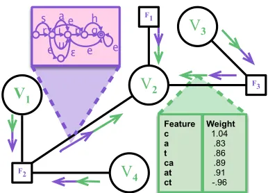
Figure 1: Information flowing towardV2 in EP (reverse
flow not shown). The factors work with purpleµ mes-sages represented by WFSAs, while the variables work with greenθmessages represented by log-linear weight vectors. The green table shows aθ message: a sparse weight vector that puts high weight on the stringcat.
EP is a variant in which all of these are forced to be log-linear functions from the same family, namelyexp(θ·fV(v)). HerefV is the featurization function we’ve chosen for variableV.3 We can rep-resent these functions by their parameter vectors— let us call thoseθV→F,θF→V, andθV respectively. 4.1 Passing messages through variables
What happens to BP’s update equations in this set-ting? According to BP, the beliefbV is the pointwise
product of all “incoming” messages toV. But as we saw in section 3.2, pointwise products arefar eas-ierin EP’s restricted setting! Instead of intersecting several WFSAs, we can simply add several vectors:
θV =
X
F0∈N(V)
θF0→V (4)
Similarly, the “outgoing” message fromV to factor F is the pointwise product of all “incoming” mes-sagesexcept the one fromF. This messageθV→F
can be computed asθV−θF→V, which adjusts (4).4
We never store this but just compute it on demand. 3A single graphical model might mix categorical variables, continuous variables, orthographic strings over (say) the Roman alphabet, and phonological strings over the International Pho-netic Alphabet. These different data types certainly require dif-ferent featurization functions. Moreover, even when two vari-ables have the same type, we could choose to approximate their marginals differently, e.g., with bigram vs. trigram features.
4.2 Passing messages through factors
Our factors are weighted finite-state machines, so their messages still require finite-state computations, as shown by the purple material in Figure 1. These computations are just as in BP. Concretely, letF be a factor of degreed, given as ad-tape machine. We can compute a beliefat this factorby joiningFwith d WFSAs that represent itsd incoming messages, namely ENCODE(θV0→F) for V0 ∈ N(F). This
gives a new d-tape machine, bF. We then obtain
each outgoing messageµF→V by projectingbF onto
itsV tape, but removing (dividing out) the weights that were contributed (multiplied in) byθV→F.5 4.3 Getting from factors back to variables
Finally, we reach the only tricky step. Each resulting µF→V is a possibly large WFSA, so we mustforce it back into our log-linear familyto get an updated ap-proximationθF→V. One cannot directly employ the
methods of section 3, because KL divergence is only defined between probability distributions. (µF→V
might not be normalizable into a distribution, nor is its best approximation necessarily normalizable.)
The EP trick is to use section 3 to instead approx-imate the belief at V, which is a distribution, and
thenreconstruct the approximate message toV that would have produced this approximated belief. The “unapproximated belief”pˆV resembles (4): it
multi-plies the unapproximated messageµF→V by the
cur-rent values of allothermessagesθF0→V. We know
the product of thoseothermessages,θV→F, so
ˆ
pV :=µF→V µV→F (5)
where the pointwise product is carried out by WFSA intersection andµV→F =def ENCODE(θV→F).
We now apply section 3 to choose θV such that qθV is a good approximation of the WFSApˆV. Fi-nally, to preserve (4) as an invariant, we reconstruct
θF→V :=θV −θV→F (6) 5This is equivalent to computing eachµ
F→V by
“general-ized composition” ofF with the d−1messages toF from itsotherneighborsV0. The operations of join and generalized composition were defined by Kempe et al. (2004).
In the simple cased = 2,F is just a weighted finite-state transducer mappingV0toV, and computingµ
F→V reduces to
composing ENCODE(θV0→F)withFand projecting the result
onto the output tape. In fact, one can assume WLOG thatd≤2, enabling the use of popular finite-state toolkits that handle at most 2-tape machines. See Appendix B.10 for the construction.
In short, EP combines µF→V with θV→F, then
approximates the resultpˆV byθV before removing θV→F again. Thus EP is approximatingµF→V by θF→V := argmin
θ D(µ|F→V {zµV→F}
= ˆpV
||q|θ{zµV→F} =θV
)
(7) in a way that updates not onlyθF→V but alsoθV.
Wisely, this objective focuses on approximating the message’s scores for the plausible values v. Some valuesv may have pˆV(v) ≈ 0, perhaps
be-causeanotherincoming messageθF0→V rules them
out. It does not much harm the objective (7) if these µF→V(v) are poorly approximated by qθF→V(v), since the overall belief is still roughly correct.
OurpenalizedEP simply addsλ·Ω(θ)into (7).
4.4 The EP algorithm: Putting it all together
To run EP (or PEP), initialize allθV andθF→V to0,
and then loop repeatedly over the nodes of the factor graph. When visiting a factorF, ENCODEits
incom-ing messagesθV→F (computed on demand) as
WF-SAs, construct a beliefbF, and update the outgoing
WFSA messagesµF→V. When visiting a variable V, iterate K ≥ 1 times over its incoming WFSA messages: for each incoming µF→V, compute the
unapproximated beliefpˆV via (5), then updateθV to
approximatepˆV, then updateθF→V via (6).
For possibly faster convergence, one can alternate “forward” and “backward” sweeps. Visit the factor graph’s nodes in a fixed order (given by an approx-imate topological sort). At a factor, update the out-going WFSA messages tolater variables only. At a variable, approximate only those incoming WFSA messages fromearlierfactors (all the outgoing mes-sagesθV→F will be recomputed on demand). Note
that both cases examine all incoming messages. Af-ter each sweep, reverse the node ordering and repeat. If gradient ascent is used to find theθV that
ap-proximatespˆV, it is wasteful to optimize to
conver-gence. After all, the optimization problem will keep changing as the messages change. Our implementa-tion improvesθV by only a single gradient step on
each visit toV, sinceV will be visited repeatedly. See Appendix A for an alternative view of EP.
5 Related Approximation Methods
vari-able’s outgoing messages are pointwise products of the incoming ones, so they become simple too. Past work has used approximations with a similar flavor. Hall and Klein (2011) heuristically predetermine a short, fixed list of plausible values forV that were observed elsewhere in their dataset. This list is anal-ogous to ourθV. After updatingµF→V, they force µF→V(v) to 0 for all v outside the list, yielding a finitemessage that is analogous to ourθF→V.
Our own past papers are similar, except they
adaptively set the “plausible values” list to S
F0∈N(V)k-BEST(µF0→V). These strings are
fa-vored by at least one of thecurrentmessages toV (Dreyer and Eisner, 2009; Dreyer and Eisner, 2011; Cotterell et al., 2015). Thus, simplifying one ofV’s incoming messages considers all of them, as in EP.
The above methodspruneeach message, so may prune correct values. Hall and Klein (2010) avoid this: they fit a full bigram model by inclusive KL divergence, which refuses to pruneanyvalues (see section 3). Specifically, they minimizedD(µF→V τ ||qθτ), whereτ was a simple fixed function (a 0-gram model) included so that they were working with distributions (see section 4.3). This is very sim-ilar to our (7). Indeed, Hall and Klein (2010) found their procedure “reminiscent of EP,” hinting that τ was a surrogate for a realµV→F term. Dreyer and
Eisner (2009) had also suggested EP as future work. EP has been applied only twice before in the NLP community. Daumé III and Marcu (2006) used EP for query summarization (following Minka and Laf-ferty (2003)’s application to an LDA model with fixed topics) and Hall and Klein (2012) used EP for rich parsing. However, these papers inferred a single structured variable connected to all factors (as in the traditional presentation of EP—see Appendix A), rather than inferring many structured variables con-nected in a sparse graphical model.
We regard EP as a generalization of loopy BP for just this setting: graphical models with large or un-bounded variable domains. Of course, we are not the first to use such a scheme; e.g., Qi (2005, chap-ter 2) applies EP to linear-chain models with both continuous and discrete hidden states. We believe that EP should also be broadly useful in NLP, since it naturally handles joint distributions over the kinds of structured variables that arise in NLP.
6 Two Methods for Optimizingθ
We now fill in details. If the feature set is defined by an unambiguous FSAA(section 3.4), two methods exist to maxEv∼p[logqθ(v)]as section 3.1 requires.
Closed-form.Determine how oftenAwould tra-verse each of its arcs, in expectation, when reading a random string drawn fromp. We would obtain an optimal ENCODE(θ) by, at each state ofA, setting
the weights of the arcs from that state to be propor-tional to these counts while summing to 1.6 Thus, the logs of these arc weights give an optimalθ.
For example, in a trigram model, the probability of thecarc from theabstate is the expected count of
abc(according to p) divided by the expected count ofab. Such expected substring counts can be found by the method of Allauzen et al. (2003). For gen-eralA, we can use the method sketched by Li et al. (2009, footnote 9): intersect the WFSA forp with the unweighted FSAA, and then run the forward-backward algorithm to determine the posterior count of each arc in the result. This tells us the expected to-tal number of traversals of each arc inA, if we have kept track of which arcs in the intersection ofpwith
Awere derived from which arcs in A. That book-keeping can be handled with an expectation semir-ing (Eisner, 2002), or simply with backpointers.
Gradient ascent. For any given θ, we can use the WFSAsp and ENCODE(θ) to exactly compute Ev∼p[logqθ(v)] = −H(p, qθ)(Cortes et al., 2006). We can tuneθto globally maximize this objective.
The technique is to intersectpwith ENCODE(θ),
after lifting their weights into the expectation semir-ing via the mappsemir-ingsk7→ hk,0iandk7→ h0,logki
respectively. Summing over all paths of this in-tersection via the forward algorithm yields hZ, ri
whereZ is the normalizing constant forp. We also sum over paths of ENCODE(θ) to get the
normal-izing constant Zθ. Now the desired objective is
r/Z−logZθ. Itsgradientwith respect toθcan be
found by back-propagation, or equivalently by the forward-backward algorithm (Li and Eisner, 2009).
An overlarge gradient step can leave the feasible space (footnote 1) by driving ZθV to ∞ and thus driving (2) to ∞ (Dreyer, 2011, section 2.8.2). In this case, we try again with reduced stepsize.
6.1 Optimizingθwith a penalty
Now consider the penalized objective (3). Ideally,
Ω(θ)would count the number of nonzero weights in
θ—or better, the number of arcs in ENCODE(θ). But
it is not known how to efficiently minimize the re-sulting discontinuous function. We give two approx-imate methods, based on the two methods above.
Proximal gradient. Leaning on recent advances in sparse estimation, we replace this Ω(θ) with a convex surrogate whose partial derivative with re-spect to eachθwis undefined atθw = 0(Bach et al.,
2011). Such a penalty tends to create sparse optima. A popular surrogate is an `1 penalty, Ω(θ) =def P
w|θw|. However, `1 would not recognize that θ is simpler with the features {ab,abc,abd} than with the features{ab,pqr,xyz}. The former leads to a smaller WFSA encoding. In other words, it is cheaper to addabdonceabcis already present, as a state already exists that represents the contextab.
We would thus like the penalty to be the number of distinctprefixesin the set of nonzero features,
|{u∈Σ∗ : (∃x∈Σ∗)θ
ux6= 0}|, (8)
as this is the number of ordinary arcs in ENCODE(θ)
(see Appendix B.4). Its convex surrogate is
Ω(θ)=def X u∈Σ∗
s X
x∈Σ∗ θ2
ux (9)
This tree-structured group lasso (Nelakanti et al., 2013) is an instance of group lasso (Yuan and Lin, 2006) where the string w = abd belongs to four groups, corresponding to its prefixes u = , u =
a, u=ab, u=abd. Under group lasso, movingθw
away from 0 increasesΩ(θ)byλ|θw|(just as in`1) for each group in which wis the only nonzero fea-ture. This penalizes for the new WFSA arcs needed for these groups. There are also increases due to w’s other groups, but these are smaller, especially for groups with many strongly weighted features.
Our objective (3) is now the sum of a differ-entiable convex function (2) and a particular non-differentiable convex function (9). We minimize it by proximal gradient (Parikh and Boyd, 2013). At each step, this algorithm first takes a gradient step as in section 6 to improve the differentiable term, and then applies a “proximal operator” to jump to
ε -0.6
a
1.2
b
0
aa
0
ab
0
ba
0
bb
0
Figure 2: Active set method, showing the infinite tree of all features for the alphabetΣ ={a, b}. The green nodes currently have non-zero weights. The yellow nodes are on the frontier and areallowedto become non-zero, but the penalty function is still keeping them at 0. The red nodes are not yet considered, forcing them to remain at 0.
a nearby point that improves the non-differentiable term. The proximal operator for tree-structured group lasso (9) can be implemented with an efficient recursive procedure (Jenatton et al., 2011).
What ifθis∞-dimensional because we allow all n-grams as features? Paul and Eisner (2012) used just this feature set in a dual decomposition algo-rithm. Like them, we rely on anactive setmethod (Schmidt and Murphy, 2010). We fixabcd’s weight at 0 untilabc’s weight becomes nonzero (if ever);7 only then does featureabcbecome “active.” Thus, at a given step, we only have to compute the gradient with respect to the currently nonzero features (green nodes in Figure 2) and their immediate children (yel-low nodes). This hierarchical inclusion technique ensures that we only consider a small, finite subset of alln-grams at any given iteration of optimization.
Closed-form with greedy growing. There are existing methods for estimating variable-order n -gram language models from data, based on either “shrinking” a high-order model (Stolcke, 1998) or “growing” a low-order one (Siivola et al., 2007).
We have designed a simple “growing” algorithm to estimate such a model from a WFSAp. It approx-imately minimizes the objective (3) whereΩ(θ) is given by (8). We enumerate alln-gramsw ∈Σ∗in
decreasing order of expected count (this can be done efficiently using a priority queue). We addwtoWif weestimatethat it will decrease the objective. Every so often, we measure theactualobjective (just as in the gradient-based methods), and we stop if it is no longer improving. Algorithmic details are given in Appendices B.8–B.9.
100 200 300 400 500 102
103
104
105
Time
(seconds
,log-scale)
Trigram EP (Gradient) Baseline Penalized EP (Gradient) Bigram EP (Gradient) Unigram EP (Gradient)
100 200 300 400 500 102
103
104
105
100 200 300 400 500 101
102
103
104
105
100 200 300 400 500 German
0.0 0.5 1.0 1.5 2.0 2.5 3.0 3.5 4.0
Cross-Entropy
(bits)
100 200 300 400 500 English
0.0 0.5 1.0 1.5 2.0 2.5 3.0 3.5 4.0
100 200 300 400 500 Dutch
[image:8.612.76.537.62.240.2]0.0 0.5 1.0 1.5 2.0 2.5 3.0 3.5 4.0
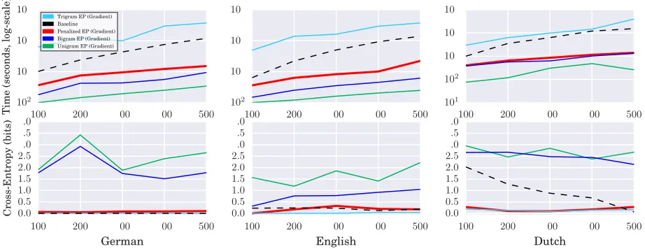
Figure 3: Inference on 15 factor graphs (3 languages ×5 datasets of different sizes). The first row shows the to-tal runtime (logscale) of each inference method. The second row shows the accuracy, as measured by the negated log-probability that the inferred belief at a variable assigns to its gold-standard value, averaged over “underlying mor-pheme” variables. At this penalty level (λ= 0.01), PEP [thick line] is faster than the pruning baseline of Cotterell et al. (2015) [dashed line] and much faster than trigram EP, yet is about as accurate. (For Dutch with sparse observations, it is considerably more accurate than baseline.) Indeed, PEP is nearly as fast as bigram EP, which has terrible accuracy. An ideal implementation of PEP would be faster yet (see Appendix B.5). Further graphs are in Appendix C.
7 Experiments and Results
Our experimental design aims to answer three ques-tions. (1) Is our algorithm able to beat a strong base-line (adaptive pruning) in a non-trivial model? (2) Is PEP actually better than ordinary EP, given that the structured sparsity penalty makes it more algo-rithmically complex? (3) Does theλparameter suc-cessfully trade off between speed and accuracy?
All experiments took place using the graphical model over strings for the discovery of underly-ing phonological forms introduced in Cotterell et al. (2015). They write: “Comparingcats([kæts]),
dogs([dOgz]), andquizzes([kwIzIz]), we see the
English plural morpheme evidently has at least three pronunciations.” Cotterell et al. (2015) sought a uni-fying account of such variation in terms of phono-logical underlying forms for the morphemes.
In their Bayes net, morpheme underlying forms are latent variables, while word surface forms are observed variables. The factors model underlying-to-surface phonological changes. They learn the fac-tors by Expectation Maximization (EM). Their first E step presents the hardest inference problem be-cause the factors initially contribute no knowledge of the language; so that is the setting we test on here.
Their data are surface phonological forms from the CELEX database (Baayen et al., 1995). For each of 3 languages, we run 5 experiments, by observ-ing the surface forms of 100 to 500 words and run-ning EP to infer the underlying forms of their mor-phemes. Each of the 15 factor graphs has≈150–700 latent variables, joined by 500–2200 edges to 200– 1200 factors of degree 1–3. Variables representing suffixes can have extremely high degree (>100).
forms). Figure 3 shows the negated log-probabilities of these gold strings according to our beliefs, aver-aged over variables in a given factor graph. Our ac-curacy is weaker than Cotterell et al. (2015) because we are doing inference with theirinitial(untrained) parameters, a more challenging problem.
Each update to θV consisted of a single step of
(proximal) gradient descent: starting at the current value, improve (2) with a gradient step of sizeη = 0.05, then (in the adaptive case) apply the proximal operator of (9) with λ = 0.01. We chose these values by preliminary exploration, taking η small enough to avoid backtracking (section 6.1).
We repeatedly visit variables and factors (sec-tion 4.4) in the forward-backward order used by Cot-terell et al. (2015). For the first few iterations, when we visit a variable we makeK = 20passes over its incoming messages, updating them iteratively to en-sure that the high probability strings in the initial ap-proximations are “in the ballpark”. For subsequent iterations of message passing we takeK = 1. For similar reasons, we constrained PEP to use only un-igram features on the first iteration, when there are still many viable candidates for each morph.
7.1 Results
The results show that PEP is much faster than the baseline pruning method, as described in Figure 3 and its caption. It mainly achieves better cross-entropy on English and Dutch, and even though it loses on German, it still places almost all of its prob-ability mass on the gold forms. While EP with un-igram and bun-igram approximations are both faster than PEP, their accuracy is poor. Trigram EP is nearly as accurate but even slower than the base-line. The results support the claim that PEP has achieved a “Goldilocks number” of n-grams in its approximation—just enough n-grams to approxi-mate the message well while retaining speed.
Figure 4 shows the effect of λ on the speed-accuracy tradeoff. To compare apples to apples, this experiment fixed the set ofµF→V messages for each
variable. Thus, we held the set of beliefs fixed, but measured the size and accuracy of different approx-imations to these beliefs by varyingλ.
These figures show only the results from gradient-based approximation. Closed-form approximation is faster and comparably accurate: see Appendix C.
102 103
Number of Features (log-scale) 0.0
0.5 1.0 1.5 2.0 2.5 3.0 3.5
Cross-Entropy
of
Gold
Standard
(bits)
λ= 0.01
λ= 0.01 λ= 0.5
[image:9.612.316.546.61.213.2]λ= 0.5 λ= 1.0 λ= 1.0
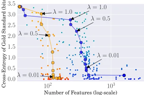
Figure 4: Increasingλ will greatly reduce the number of selected features in a belief—initially without harming accuracy, and then accuracy degrades gracefully. (Num-ber of features has 0.72 correlation with runtime, and is shown on alog scaleon thexaxis.)
Each point shows the result of using PEP to approxi-mate the belief at some latent variableV, usingµF→V
messages from running the baseline method on German. Lighter points use larger λ. Orange points are affixes (shorter strings), blue are stems (longer strings). Large circles are averages over all points for a givenλ.
8 Conclusion and Future Work
We have presented penalized expectation propaga-tion (PEP), a novel approximate inference algo-rithm for graphical models, and developed specific techniques for string-valued random variables. Our method integrates structured sparsity directly into inference. Our experiments show large speedups over the strong baseline of Cotterell et al. (2015).
In future, instead of choosing λ, we plan to re-duceλas PEP runs. This serves to gradually refine the approximations, yielding an anytime algorithm
whose beliefs approach the BP beliefs. Thanks to (7), the coarse messages from early iterations guide the choice of finer-grained messages at later itera-tions. In this regard, “Anytime PEP” resembles other coarse-to-fine architectures such as generalized A* search (Felzenszwalb and McAllester, 2007).
References
Cyril Allauzen, Mehryar Mohri, and Brian Roark. 2003. Generalized algorithms for constructing statistical lan-guage models. InProceedings of ACL, pages 40–47. Cyril Allauzen, Michael Riley, Johan Schalkwyk,
Woj-ciech Skut, and Mehryar Mohri. 2007. OpenFst: A general and efficient weighted finite-state transducer library. InProceedings of the 12th International Con-ference on Implementation and Application of Au-tomata, volume 4783 ofLecture Notes in Computer Science, pages 11–23. Springer.
R. Harald Baayen, Richard Piepenbrock, and Leon Gu-likers. 1995. The CELEX lexical database on CD-ROM.
Francis Bach, Rodolphe Jenatton, Julien Mairal, Guil-laume Obozinski, et al. 2011. Convex optimization with sparsity-inducing norms. In S. Sra, S. Nowozin, and S. J. Wright, editors, Optimization for Machine Learning. MIT Press.
Alexandre Bouchard-Côté, Percy Liang, Thomas L Grif-fiths, and Dan Klein. 2007. A probabilistic approach to diachronic phonology. InProceedings of EMNLP-CoNLL, pages 887–896.
Alexandre Bouchard-Côté, Percy Liang, Thomas Grif-fiths, and Dan Klein. 2008. A probabilistic approach to language change. InProceedings of NIPS.
Victor Chahuneau. 2013. PyFST. https:// github.com/vchahun/pyfst.
Corinna Cortes, Mehryar Mohri, Ashish Rastogi, and Michael D Riley. 2006. Efficient computation of the relative entropy of probabilistic automata. In
LATIN 2006: Theoretical Informatics, pages 323–336. Springer.
Ryan Cotterell, Nanyun Peng, and Jason Eisner. 2014. Stochastic contextual edit distance and probabilistic FSTs. InProceedings of ACL, pages 625–630. Ryan Cotterell, Nanyun Peng, and Jason Eisner. 2015.
Modeling word forms using latent underlying morphs and phonology. Transactions of the Association for Computational Linguistics. To appear.
Hal Daumé III and Daniel Marcu. 2006. Bayesian query-focused summarization. InProceedings of ACL, pages 305–312.
Markus Dreyer and Jason Eisner. 2009. Graphical mod-els over multiple strings. InProceedings of EMNLP, pages 101–110, Singapore, August.
Markus Dreyer and Jason Eisner. 2011. Discover-ing morphological paradigms from plain text usDiscover-ing a Dirichlet process mixture model. In Proceedings of EMNLP, pages 616–627, Edinburgh, July.
Markus Dreyer. 2011. A Non-Parametric Model for the Discovery of Inflectional Paradigms from Plain Text
Using Graphical Models over Strings. Ph.D. thesis, Johns Hopkins University, Baltimore, MD, April. Jason Eisner. 2002. Parameter estimation for
probabilis-tic finite-state transducers. In Proceedings of ACL, pages 1–8.
C.C. Elgot and J.E. Mezei. 1965. On relations defined by generalized finite automata. IBM Journal of Research and Development, 9(1):47–68.
Gal Elidan, Ian Mcgraw, and Daphne Koller. 2006. Residual belief propagation: Informed scheduling for asynchronous message passing. In Proceedings of UAI.
P. F. Felzenszwalb and D. McAllester. 2007. The gen-eralized A* architecture. Journal of Artificial Intelli-gence Research, 29:153–190.
David Hall and Dan Klein. 2010. Finding cognate groups using phylogenies. InProceedings of ACL. David Hall and Dan Klein. 2011. Large-scale cognate
recovery. InProceedings of EMNLP.
David Hall and Dan Klein. 2012. Training factored PCFGs with expectation propagation. InProceedings of EMNLP.
Rodolphe Jenatton, Julien Mairal, Guillaume Obozinski, and Francis Bach. 2011. Proximal methods for hierar-chical sparse coding. The Journal of Machine Learn-ing Research, 12:2297–2334.
André Kempe, Jean-Marc Champarnaud, and Jason Eis-ner. 2004. A note on join and auto-intersection of n-ary rational relations. In Loek Cleophas and Bruce Watson, editors,Proceedings of the Eindhoven FASTAR Days (Computer Science Technical Report 04-40), pages 64–78. Department of Mathematics and Computer Science, Technische Universiteit Eind-hoven, Netherlands, December.
Kevin Knight and Jonathan Graehl. 1998. Machine transliteration.Computational Linguistics, 24(4). F. R. Kschischang, B. J. Frey, and H. A. Loeliger. 2001.
Factor graphs and the sum-product algorithm. IEEE Transactions on Information Theory, 47(2):498–519, February.
Zhifei Li and Jason Eisner. 2009. First- and second-order expectation semirings with applications to minimum-risk training on translation forests. InProceedings of EMNLP, pages 40–51.
Zhifei Li, Jason Eisner, and Sanjeev Khudanpur. 2009. Variational decoding for statistical machine transla-tion. InProceedings of ACL, pages 593–601.
André F. T. Martins, Noah A. Smith, Pedro M. Q. Aguiar, and Mário A. T. Figueiredo. 2011. Structured sparsity in structured prediction. In Proceedings of EMNLP, pages 1500–1511.
Thomas Minka and John Lafferty. 2003. Expectation-propagation for the generative aspect model. In Pro-ceedings of UAI.
Thomas P Minka. 2001a. Expectation propagation for approximate Bayesian inference. In Proceedings of UAI, pages 362–369.
Thomas P. Minka. 2001b. A Family of Algorithms for Approximate Bayesian Inference. Ph.D. thesis, Mas-sachusetts Institute of Technology, January.
Thomas Minka. 2005. Divergence measures and mes-sage passing. Technical Report MSR-TR-2005-173, Microsoft Research, January.
Mehryar Mohri, Fernando Pereira, and Michael Ri-ley. 2002. Weighted finite-state transducers in speech recognition. Computer Speech & Language, 16(1):69–88.
Mehryar Mohri. 2000. Minimization algorithms for se-quential transducers. Theoretical Computer Science, 324:177–201, March.
Mehryar Mohri. 2005. Local grammar algorithms. In Antti Arppe, Lauri Carlson, Krister Lindèn, Jussi Pi-itulainen, Mickael Suominen, Martti Vainio, Hanna Westerlund, and Anssi Yli-Jyrä, editors,Inquiries into Words, Constraints, and Contexts: Festschrift in Hon-our of Kimmo Koskenniemi on his 60th Birthday, chap-ter 9, pages 84–93. CSLI Publications, Stanford Uni-versity.
Kevin P. Murphy, Yair Weiss, and Michael I. Jordan. 1999. Loopy belief propagation for approximate in-ference: An empirical study. InProceedings of UAI, pages 467–475.
Anil Nelakanti, Cédric Archambeau, Julien Mairal, Fran-cis Bach, Guillaume Bouchard, et al. 2013. Structured penalties for log-linear language models. In Proceed-ings of EMNLP, pages 233–243.
Neal Parikh and Stephen Boyd. 2013. Proximal al-gorithms. Foundations and Trends in Optimization, 1(3):123–231.
Michael Paul and Jason Eisner. 2012. Implicitly inter-secting weighted automata using dual decomposition. InProceedings of NAACL-HLT, pages 232–242, Mon-treal, June.
Judea Pearl. 1988. Probabilistic Reasoning in Intelli-gent Systems: Networks of Plausible Inference. Mor-gan Kaufmann, San Mateo, California.
Fernando C. N. Pereira and Michael Riley. 1997. Speech recognition by composition of weighted finite au-tomata. In Emmanuel Roche and Yves Schabes, ed-itors, Finite-State Language Processing. MIT Press, Cambridge, MA.
Slav Petrov, Leon Barrett, Romain Thibaux, and Dan Klein. 2006. Learning accurate, compact, and inter-pretable tree annotation. InProceedings of COLING-ACL, pages 433–440, July.
Yuan Qi. 2005. Extending Expectation Propagation for Graphical Models. Ph.D. thesis, Massachusetts Insti-tute of Technology, February.
Dana Ron, Yoram Singer, and Naftali Tishby. 1996. The power of amnesia: Learning probabilistic automata with variable memory length. Machine Learning, 25(2-3):117–149.
Mark W Schmidt and Kevin P Murphy. 2010. Convex structure learning in log-linear models: Beyond pair-wise potentials. In Proceedings of AISTATS, pages 709–716.
Vesa Siivola, Teemu Hirsimäki, and Sami Virpioja. 2007. On growing and pruning Kneser-Ney smoothed n -gram models. IEEE Transactions on Audio, Speech, and Language Processsing, 15(5):1617–1624. Andreas Stolcke. 1998. Entropy-based pruning of
backoff language models. In Proceedings of the DARPA Broadcast News Transcription and Under-standing Workshop, pages 270–274.