FBK-HLT-NLP at SemEval-2016 Task 2: A Multitask, Deep Learning
Approach for Interpretable Semantic Textual Similarity
Simone Magnolini Fondazione Bruno Kessler
University of Brescia Brescia, Italy [email protected]
Anna Feltracco Fondazione Bruno Kessler
University of Pavia Pavia, Italy [email protected]
Bernardo Magnini Fondazione Bruno Kessler
Povo-Trento, Italy [email protected]
Abstract
We present the system developed at FBK for the SemEval 2016 Shared Task 2 ”Inter-pretable Semantic Textual Similarity” as well as the results of the submitted runs. We use a single neural network classification model for predicting the alignment at chunk level, the re-lation type of the alignment and the similar-ity scores. Our best run was ranked as first in one the subtracks (i.e. raw input data, Student Answers), among 12 runs submitted, and the approach proved to be very robust across the different datasets.
1 Introduction
The Semantic Textual Similarity (STS) task mea-sures the degree of equivalence between the mean-ing of two texts, usually sentences. In the Inter-pretable STS (iSTS) (Agirre et al., 2016) the sim-ilarity is calculated at chunk level, and systems are asked to provide the type of the relationship between two chunks, as an interpretation of the similarity. Given an input pair of sentences, participant sys-tems were asked to: (i) identify the chunks in each sentence; (ii) align chunks across the two sentences; (iii) indicate the relation between the aligned chunks and (iv) specify the similarity score of each align-ment.
The iSTS task has already been the object of an evaluation campaign in 2015, as a subtask of the SemEval-2015 Task 2: Semantic Textual Similarity (Agirre et al., 2015). More in general, shared tasks for the identification and measurement of STS were organized in 2012 (Agirre et al., 2012), 2013 (Agirre et al., 2013) and 2014 (Agirre et al., 2014).
Data provided to participants include three datasets: image captions (Images), pairs of sen-tences from news headlines (Headlines), and a question-answer dataset collected and annotated during the evaluation of the BEETLE II tutorial dialogue system (Student Answers) (Agirre et al., 2015). For each dataset, two subtracks were re-leased: the first with raw input data (SYS), the sec-ond with data split in gold standard chunks (GS). Given these input data, participants were required to identify the chunks in each sentence (for the first subtrack only), align chunks across the two sen-tences, specify the semantic relation of the align-ment - selecting one of the following: EQUI for equivalent, OPPO for opposite, SPE1 and SPE2 if chunk in sentence1 is more specific than chunk in sentence2 and vice versa, SIMI for similar mean-ings, REL for chunks that have related meanmean-ings, and NOALI for chunk has no corresponding chunk in the other sentence (Agirre et al., 2015)-, and pro-vide a similarity score for each alignment, from 5 (maximum similarity/relatedness) to 0 (no relation at all). In addition, an optional tag for alignments showing factuality (FACT) or polarity (POL) phe-nomena, can be specified. The evaluation is based on (Melamed, 1998), which uses the F1 of precision and recall of token alignments.
We participate in the iSTS shared task with a system that combines different features - includ-ing word embeddinclud-ing and chunk similarity - usinclud-ing a Multilayer Perceptrons (MLP). Our main contri-bution was focused on the optimization of a Neural Network setting (i.e. topology, activation function, multi-task training) for the iSTS task. We show that
even with a relatively small and unbalanced training dataset, a neural network classifier can be built that achieves results very close to the best system. Par-ticularly, our system makes use of a single model for the different training sets of the task, proving to be very robust to domain differences.
The paper is organized as follows. Section 2 presents the system we built; Section 3 reports the results we obtained and an evaluation of our system. Finally, Section 4 provides some conclusions.
2 System Description
Our system is built combining different linguis-tic features in a classification model for predicting chunk-to-chunk alignment, relation type and STS score. We decide to use the same features for all these three subtasks and to use a unique multitask MLP with shared layers for all the subtasks. The system is expandable and scalable for adopting more useful features aiming at improving the accuracy.
In this Section, we describe the pre-processing of the data, the features we used, the MLP structure, its training, its output and, finally, the difference be-tween the three submitted runs.
2.1 Data Pre-processing
The input data undergo a data pre-processing in which we use a Python implementation of MBSP (Daelemans and Van den Bosch, 2005), a library providing tools for tokenization, sentence splitting, part of speech tagging, chunking, lemmatization and prepositional phrase attachment. The MBSP chun-ker is used in the SYS subtrack, which requires par-ticipants to identify the chunks in each sentence. For both subtracks, we pre-processed the initial datasets of sentence pairs by pairing all the chunks in the first sentence with all the chunks in the second sentence. Henceforth, we will refer to the two chunks in each of the obtained pairs aschunk1 and chunk2, being
chunk1 a chunk of the first sentence and chunk2 a chunk of the second sentence.
2.2 Feature Selection
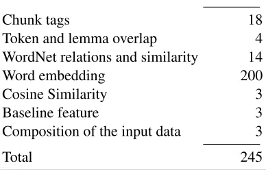
To compute the chunk-to-chunk alignment, the relation type and the STS score we use a total of 245 features.
Chunk tags. A total of 18 features (9 forchunk1
and 9 for chunk2) are related to chunk tags (e.g. noun phrase, prepositional phrase, verb phrase).
For each chunk in the SYS datasets -chunked with MBSP- the system takes into consideration the chunk tags as identified by that library.1
For the GS datasets -already chunked datasets- the system first re-chunks the datasets with MBSP and than evaluates if chunks in the GS corresponds to chunks as identified in MBSP. If this is the case, chunk tag is extracted; otherwise the systems does the same operation (i.e. re-chunking and tag extrac-tion) using pattern.en (De Smedt and Daelemans, 2012), a regular expressions-based shallow parser for English that uses a part-of-speech tagger ex-tended with a tokenizer, lemmatizer and chunker.2
If no corresponding chunk is found, no chunk tag is assigned.
Token and lemma overlap. Four further fea-tures are related to tokens and lemmas overlap between a pair of chunks. In particular, the system considers the percentage of (i) tokens and (ii) lemmas in chunks1 that are present also inchunk2
and viceversa (iii - iv).
WordNet based features. Another group of features concerns lexical and semantic relations between words extracted from WordNet 3.0 (Fell-baum, 1998). As such, we evaluate the type of relation between chunks by considering all the lemmas in the two chunks and checking whether a lemma inchunk1is a synonym, antonym, hyponym, hyperonym, meronym or holonym of a lemma in
chunk2. The relations between all the combinations of the lemmas in the two chunks are extracted. The presence or absence of a relation is consider a feature at chunk level (for a total of 6 features for
chunk1and 6 features forchunk2).
Furthermore, we consider as a feature the synset similarity existing in the WordNet hierarchy be-tween each lemma in the two chunks, as calculated
1The chunk tags are the following: noun phrase (NP), prepo-sitional phrase (PP), verb phrase (VP), adverb phrase (ADVP), adjective phrase (ADJP), subordinating conjunction (SBAR), particle (PRT), interjection (INTJ), prepositional noun phrase (PNP).
by pattern.en. We calculate the average of the best alignments for each lemma in the two chunks. For example, consider the chunk pair: chunk1
”the animal” and chunk2 ”the sweet dog”. For each lemma in chunk1, for which a synset can be retrieved from WordNet, (”animal”), we calculate the maximum similarity with lemmas in chunk2. Thus, for this pair of chunks the resulting maximum similarity is between ”animal-dog” = 0.299 (being equal to 0.264 for ”animal-sweet”). The chunk similarity score is 0.299. With the same strategy we calculate similarity between lemmas in chunk2
towardschunk1, i.e. ”sweet-animal” = 0.264 , ”dog-animal” = 0.299 resulting in a chunk similarity score of [(0.264 + 0.299)/ 2] = 0.281. If lemmas were not found in WordNet, the synset similarity is considered 0.
Word embedding. We use a distributional representation of the chunk for a total of 200 fea-tures (100 for chunk1 and 100 for chunk2) by first calculating word embedding and then combining the vectors of the words in the chunk (i.e. by calculating the element wise mean of each vector). We use Mikolov word2vec (Mikolov et al., 2013) with 100 dimensions using ukWaC, GigaWords (NYT), Europarl V.7, Training Set (JRC) corpora.
The system computes the chunk-to-chunk simi-larity by calculating the cosine simisimi-larity between the two chunk vectors with three different models: the first uses the already described vectors (one feature); the second uses vectors representations extracted with a different corpus and a different parametres -i.e. Google News, with 300 dimensions of the vectors- (one feature); the third uses GloVe vectors (Pennington et al., 2014) with 300 dimen-sions (one feature).
Baseline feature. The baseline output - pro-vided by the organizers (Agirre et al., 2016) - was also exploited, i.e. we consider if the chunks are evaluated as aligned, if chunk1 is not aligned, if
chunk2is not aligned (3 features).
Composition of the input data. The last three features refer to the datasets. The system takes into consideration if the chunks are extracted from Headline, Images, or Student Answers dataset.
#features
Chunk tags 18
Token and lemma overlap 4 WordNet relations and similarity 14
Word embedding 200
Cosine Similarity 3
Baseline feature 3
Composition of the input data 3
[image:3.612.330.524.75.199.2]Total 245
Table 1:Feature Selection.
2.3 Neural Network
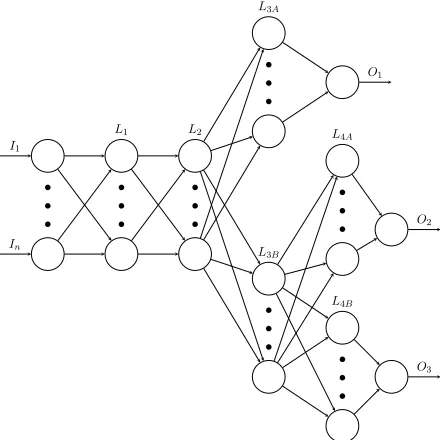
We use a multitask MLP (see Figure 1) to classify chunk pairs, implemented with the TensorFlow li-brary (Abadi et al., 2015). The system uses three classifiers: one for the chunk alignment, one for alignment type, one for STS score. The input layer has 245 entities, so we use fully connected hidden layers with 250 nodes. During the test we observed that smaller (200 nodes) or bigger (300 nodes) layers reduce the performances. The system is composed by two layers (i.e. L1 and L2) shared between the three classifiers. On the top of them there are other two layers: the former (L3a) used only for the align-ment classifier and the latter (L3b) shared among the score classifier and the type classifier. At the very end of L3b, there are other two layers one for the score (L4a) and one for the type (L4b). In synthe-sis for alignment there are three hidden layers, two shared (L1 and L2) and one private (L3a), for STS score there are four hidden layers, three shared (L1, L2, L3b) and one private (L4a) and the same for the type labeling (L1, L2, L3b + L4b). Every output lay-ers is a softmax; during the training the system has a dropout layer that remove nodes from the layer with a probability of 50% to avoid overfitting.
... ... ...
...
...
...
...
I1
In
L1 L2
L3A
L3B
L4A
L4B
O1
O2
[image:4.612.84.304.62.282.2]O3
Figure 1:Multitask learning Neural Network.
the other ones.
We train the classifiers for three cycles. This train-ing strategy is driven by learntrain-ing curves analysis: we keep training the classifiers until the learning curves keep growing. We notice that the alignment classi-fier stops learning earlier, followed by the relation type classifier, and, at the end, the STS score classi-fier. Under these findings, to train all the classifiers in the same way overfits the training data. Further-more, the training data are very unbalanced (most of the pairs are not aligned); thus, we use random mini-batches with a fix proportion between aligned pairs and unaligned pairs. To do so, we use the unaligned pairs more than once in a single training epoch. In particular, first we train the alignment classifier with the following proportion: 2/5 of aligned examples and 3/5 of not aligned pairs, for 8 training epochs (i.e. every aligned pair is used as training data at least 8 times). The second training cycle optimizes relation type labeling and STS score, with the pro-portion of 9/10 aligned and 1/10 not aligned for other 8 training epochs. Finally, in the third training cyle, we train only for STS score with a proportion of 9/10 aligned and 1/10 not aligned pairs.
2.4 Output
We combine the output of the three classifiers (align-ment, relation type and similarity score) organized
in a pipeline. First, we label as ”not aligned” all the punctuation chunks (i.e. those defined as ”not alignable” by the baseline); then we label as ”aligned” all the chunks aligned by the first classi-fier, allowing multiple alignments for each chunk. For every aligned chunk pair we add the type label and the STS score. We do not take into consider-ation chunk pairs classified as ”not aligned” by the first classifier even if they are classified with a label different from NOTALI or with an STS score higher than 0.
2.5 Submitted Runs
We submitted three runs, with different training set-tings. In the first run we use all the training data with a mini-batch of 150 elements. In the second run we train and evaluate separately each dataset with a mini-batch of 150 elements. Finally, in the third run we use all the training data with a mini-batch of 200 elements. We choose these settings in order to eval-uate how in-domain data and different sizes of the mini-batch influence the classification results.
3 Results and Evaluation
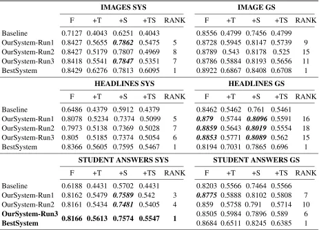
Table 2 compares the results of our runs with the baseline and the best system for each subtrack of the three datasets, showing:
• F1 on alignment classification (F);
• F1 on alignment classification plus relation alignment type (+T);
• F1 on alignment classification plus STS score (+S);
• F1 on alignment classification plus relation alignment type and STS score (+TS);
• Ranked position over the runs submitted: i.e.
13 runs for Images and Headlines SYS, 12 for Student Answer SYS, 20 for Images and Headlines GS and 19 for Student Answer GS (RANK)
IMAGES SYS IMAGE GS
F +T +S +TS RANK F +T +S +TS RANK
Baseline 0.7127 0.4043 0.6251 0.4043 0.8556 0.4799 0.7456 0.4799 OurSystem-Run1 0.8427 0.5655 0.7862 0.5475 5 0.8728 0.5945 0.8147 0.5739 9 OurSystem-Run2 0.8427 0.5179 0.7807 0.4969 8 0.8789 0.543 0.8178 0.525 15 OurSystem-Run3 0.8418 0.5541 0.7847 0.5351 7 0.8786 0.5884 0.8193 0.5656 11 BestSystem 0.8429 0.6276 0.7813 0.6095 1 0.8922 0.6867 0.8408 0.6708 1
HEADLINES SYS HEADLINES GS
F +T +S +TS RANK F +T +S +TS RANK
Baseline 0.6486 0.4379 0.5912 0.4379 0.8462 0.5462 0.761 0.5461 OurSystem-Run1 0.8078 0.5234 0.7374 0.5099 5 0.879 0.5744 0.8096 0.5591 16 OurSystem-Run2 0.7973 0.5138 0.7369 0.5028 7 0.8859 0.5643 0.8019 0.5554 18 OurSystem-Run3 0.805 0.5185 0.7374 0.5054 6 0.8853 0.5771 0.8089 0.562 15 BestSystem 0.8366 0.5605 0.7595 0.5467 1 0.8194 0.7031 0.7865 0.696 1
STUDENT ANSWERS SYS STUDENT ANSWERS GS
F +T +S +TS RANK F +T +S +TS RANK
Baseline 0.6188 0.4431 0.5702 0.4431 0.8203 0.5566 0.7464 0.5566 OurSystem-Run1 0.8162 0.5479 0.7589 0.542 3 0.8775 0.5888 0.8102 0.5808 7 OurSystem-Run2 0.8161 0.5434 0.7481 0.5405 4 0.859 0.5758 0.791 0.5714 10
OurSystem-Run3 0.8166 0.5613 0.7574 0.5547 1 0.8505 0.5984 0.7896 0.589 6
[image:5.612.75.538.60.394.2]BestSystem 0.8684 0.6511 0.8245 0.6385 1
Table 2:Results for the Baseline, Our System three runs and the Best System for the two subtracks split in the three datasets.
suggest that the system takes advantage of a bigger training set with different domain data. Instead, the size of the mini-batch (that is the difference between run1 and run3) does not seem to have a clear influ-ence on the system performance, since in some cases run1 is higher ranked while in other cases run3 is higher ranked.
Furthermore, Table 2 shows that results for Align-ment classification (F) and for AlignAlign-ment plus STS score (+S) frequently approach the Best System (be-ing the major deficit for F equal to 0.0393 in Head-line SYS for run3 and equal to 0.0349 for +S in Student Answwer GS dataset for run3) and in a few cases outperform it (e.g. in Headlines GS for F re-sults and in Images SYS for +S rere-sults). On the other hand, when also relation type classification is considered (i.e. +T and +TS) we register worse per-formances, being the minimum difference with the Best System equals to 0.0371 for +T results and of 0.0368 for +TS results (both in Headlines SYS) and
the maximum difference equals to 0.1437 for +T and to 0.1458 for +TS (both in Images GS). This indi-cates that type labelling is the hardest subtask for our system, probably because the subtask requires to identify a higher number of classes (i.e. 7 types).
By comparing the rank of the two subtracks SYS and GS, we notice that our system performs much better in the SYS subtrack (being the worst ranking 8 out of 13 for SYS and 18 out of 20 for GS). This fact indicates that our system does not benefit from having already chunked sentence pairs.
SYS GS MEAN RANK MEAN RANKF + TS F + TS
[image:6.612.73.281.61.182.2]Baseline 0.428433 0.527533 Run1 0.533133 4 0.571266 11 Run2 0.5134 6 0.5506 17 Run3 0.531733 5 0.5722 10 BestSystem 0.552333 1 0.637733 1
Table 3:Mean of the F+TS results in the two subtracks for the Baseline, Our System three runs and the Best System and final rank.
4 Conclusion and Further Work
Considering the obtained results, in particular the difference between the runs, we expect our system to be robust also in situation where data from dif-ferent domains are provided (e.g. training data from several domains and test data on one of them). In fact, for domain adaptation our system seems to re-quire few data of the target domain.
In any case, the system perform better with more training data, independently on the domains in-volved. As such, further work may include the use of silver data extracted from other datasets, e.g. SICK dataset (Marelli et al., 2014).
In addition, we believe that a deep analysis of the distribution of the type labels and of the STS scores can improve significantly the performance of the system.
Finally, an ablation test can be helpful in identify-ing the most salient features for the systems, helpidentify-ing to reduce the complexity of the MLP or to develop better topologies.
Acknowledgments
We are grateful to Jos´e G. C. de Souza, Matteo Ne-gri, and Marco Turchi for their suggestions.
References
Mart´ın Abadi, Ashish Agarwal, Paul Barham, Eugene Brevdo, Zhifeng Chen, Craig Citro, Greg S. Corrado, Andy Davis, Jeffrey Dean, Matthieu Devin, Sanjay Ghemawat, Ian Goodfellow, Andrew Harp, Geoffrey Irving, Michael Isard, Yangqing Jia, Rafal Jozefow-icz, Lukasz Kaiser, Manjunath Kudlur, Josh Leven-berg, Dan Man´e, Rajat Monga, Sherry Moore, Derek
Murray, Chris Olah, Mike Schuster, Jonathon Shlens, Benoit Steiner, Ilya Sutskever, Kunal Talwar, Paul Tucker, Vincent Vanhoucke, Vijay Vasudevan, Fer-nanda Vi´egas, Oriol Vinyals, Pete Warden, Martin Wattenberg, Martin Wicke, Yuan Yu, and Xiaoqiang Zheng. 2015. TensorFlow: Large-scale machine learning on heterogeneous systems. Software avail-able from tensorflow.org.
Eneko Agirre, Mona Diab, Daniel Cer, and Aitor Gonzalez-Agirre. 2012. Semeval-2012 task 6: A pilot on semantic textual similarity. InProceedings of the First Joint Conference on Lexical and Computational Semantics-Volume 1: Proceedings of the main confer-ence and the shared task, and Volume 2: Proceedings of the Sixth International Workshop on Semantic Eval-uation, pages 385–393. Association for Computational Linguistics.
Eneko Agirre, Daniel Cer, Mona Diab, Aitor Gonzalez-Agirre, and Weiwei Guo. 2013. sem 2013 shared task: Semantic Textual Similarity, including a Pilot on Typed-Similarity. InIn* SEM 2013: The Second Joint Conference on Lexical and Computational Semantics. Association for Computational Linguistics. Citeseer. Eneko Agirre, Carmen Banea, Claire Cardie, Daniel
Cer, Mona Diab, Aitor Gonzalez-Agirre, Weiwei Guo, Rada Mihalcea, German Rigau, and Janyce Wiebe. 2014. Semeval-2014 task 10: Multilingual Semantic Textual Similarity. In Proceedings of the 8th Inter-national Workshop on Semantic Evaluation (SemEval 2014), pages 81–91.
Eneko Agirre, Carmen Baneab, Claire Cardiec, Daniel Cerd, Mona Diabe, Aitor Gonzalez-Agirrea, Wei-wei Guof, Inigo Lopez-Gazpioa, Montse Maritxalara, Rada Mihalceab, et al. 2015. Semeval-2015 task 2: Semantic Textual Similarity, English, Spanish and Pi-lot on Interpretability. InProceedings of the 9th Inter-national Workshop on Semantic Evaluation (SemEval 2015), pages 252–263.
Eneko Agirre, Aitor Gonzalez-Agirre, I˜nigo Lopez-Gazpio, Montse Maritxalar, German Rigau, and Lar-raitz Uria. 2016. Semeval-2016 task 2: Interpretable semantic textual similarity. InProceedings of the 10th International Workshop on Semantic Evaluation (Se-mEval 2016), San Diego, California, June.
Walter Daelemans and Antal Van den Bosch. 2005.
Memory-based language processing. Cambridge Uni-versity Press.
Tom De Smedt and Walter Daelemans. 2012. Pattern for python. The Journal of Machine Learning Research, 13(1):2063–2067.
Christiane Fellbaum. 1998. WordNet. Wiley Online Li-brary.
method for stochastic optimization. arXiv preprint arXiv:1412.6980.
Marco Marelli, Stefano Menini, Marco Baroni, Luisa Bentivogli, Raffaella Bernardi, and Roberto Zampar-elli. 2014. A sick cure for the evaluation of compo-sitional distributional semantic models. In Proceed-ing of Language Resources and Evaluation Confer-ence (LREC 2014), pages 216–223.
I. Dan Melamed. 1998. Manual annotation of trans-lational equivalence: The blinker project. Technical Report 98-07, Institute for Research in Cognitive Sci-ence, Philadelphia.
Tomas Mikolov, Ilya Sutskever, Kai Chen, Greg S Cor-rado, and Jeff Dean. 2013. Distributed representa-tions of words and phrases and their compositionality. InAdvances in neural information processing systems, pages 3111–3119.