Gradual Learning of Matrix-Space Models of Language
for Sentiment Analysis
Shima Asaadi∗and Sebastian Rudolph
Faculty of Computer Science TU Dresden, Germany [email protected]
Abstract
Learning word representations to capture the semantics and compositionality of language has received much research interest in natu-ral language processing. Beyond the popu-lar vector space models, matrix representations for words have been proposed, since then, ma-trix multiplication can serve as natural com-position operation. In this work, we investi-gate the problem of learning matrix representa-tions of words. We present a learning approach for compositional matrix-space models for the task of sentiment analysis. We show that our approach, which learns the matrices gradually in two steps, outperforms other approaches and a gradient-descent baseline in terms of quality and computational cost.
1 Introduction
Recently, a lot of NLP research has been de-voted to word representations with the goal to capture language semantics, compositionality, and other linguistic aspects. A prominent class of approaches to produce word representations are Vector Space Models (VSMs) of language. In VSMs, a vector representation is created for each word in the text, mostly based on distributional information. One of the recent prominent meth-ods to extract vector representations of words is Word2vec, introduced by Mikolov et al. (2013a;
2013b). These models measure both syntactic and semantic aspects of words and also seem to exhibit good compositionality properties. The principle of compositionality states that the meaning of a complex expression can be obtained from combin-ing the meancombin-ing of its constituents (Frege,1884). In the Word2vec case and many other VSM ap-proaches, some vector space operations (such as ∗Supported by DFG Graduiertenkolleg 1763 (QuantLA)
vector addition) are used as composition opera-tion.
One of the downsides of using vector addi-tion (or other commutative operaaddi-tions like the component-wise product) as the compositional-ity operation is that word order information is inevitably lost. Alternative word-order-sensitive compositionality models for word representations have been introduced, such as Compositional Matrix-Space Models (CMSMs) (Rudolph and Giesbrecht, 2010). In such models, matrices in-stead of vectors are used as word representations and compositionality is realized via matrix mul-tiplication. It has been proven that CMSMs are capable of simulating a wide range of VSM-based compositionality operations. The question, how-ever, how to learn suitable word-to-matrix map-pings has remained largely unexplored with few exceptions (Yessenalina and Cardie, 2011). The task is exacerbated by the fact that this amounts to a non-convex optimization problem, where a good initialization is crucial for the success of gradient descent techniques.
In this paper, we address the problem of learn-ing CMSM in the domain of sentiment analysis. As has been observed before, the sentiment of a phrase is very much influenced by the presence and position of negators and modifiers, thus word order seems to be particularly relevant for estab-lishing an accurate sentiment score.
We propose to apply a two-step learning method where the output of the first step serves as ini-tialization for the second step. We evaluate the performance of our method on the task of fine-grained sentiment analysis and compare it to a previous work on learning CMSM for sentiment analysis (Yessenalina and Cardie, 2011). More-over, the performance of our representation learn-ing in sentiment composition is evaluated on sen-timent composition in opposing polarity phrases
(Kiritchenko and Mohammad,2016b).
The rest of the paper is organized as follows. Section 2 provides the related works. A detailed description of the approach is presented in Section 3, followed by experiments and discussion in Sec-tion 4, and the conclusion in the last secSec-tion.
2 Related Work
Compositional Distributional Semantics: In compositional distributional semantics, different approaches for learning word and phrase represen-tations and ways to compose the constituents are studied. As an early work in compositional dis-tributional semantics, Mitchell and Lapata(2010) propose vector composition models with additive and multiplicative functions as the composition operations in semantic VSMs. These models out-perform non-compositional approaches in seman-tic similarity of complex expressions. Mikolov et al. (2013a) propose Word2vec where contin-uous vector representations of words are trained through continuous bag-of-words and skip-gram models. These models are supposed to reflect syntactic and semantic similarities of words. An extension to these models is a vector representa-tion of idiomatic phrases by considering a vec-tor for each phrase and training Word2vec accord-ingly (Mikolov et al.,2013b). Moreover, compo-sitionality is captured in these models by applying certain mathematical operations on word vectors.
Rudolph and Giesbrecht (2010) introduced compositional matrix-space models in which words are represented as matrices, and defined composition operation as a matrix multiplication function. Learning such matrix representations can be done by supervised machine learning al-gorithms (Yessenalina and Cardie, 2011). Other approaches using matrices for distributional rep-resentations of words have been introduced more recently.Socher et al.(2012) introduce a model in which a matrix and a vector is assigned to each word. The vector captures the meaning of the word by itself and the matrix shows how it modi-fies the meaning of neighboring words. The model is learned through recursive neural networks. In the model ofSocher et al.(2013), a unique tensor-based composition function in a recursive neural tensor network is introduced which composes all word vectors. Maillard and Clark(2015) describe a compositional model for learning adjective-noun pairs where, first, a vector representation for each
word is trained using a skip-gram model. Then, adjective matrices are trained in composition to their nouns, using back-propagation.
Sentiment Analysis:There is a lot of research in-terest in the sentiment analysis task in NLP. The task is to classify the polarity of a text (negative, positive, neutral) or assign a real-valued score, showing the polarity and intensity of the text. Some contributions focus on learning sentiment of a short text based on supervised machine learn-ing techniques (Yessenalina and Cardie, 2011;
Agrawal and An,2014). Recent approaches have focused on learning different types of neural net-works for sentiment analysis, such as the work ofSocher et al.(2013) which apply recursive neu-ral tensor networks for both fine-grained and bi-nary classification of phrases and sentences. Tim-maraju and Khanna(2015) use recursive-recurrent neural networks for sentiment classification of long text, andHong and Fang(2015) apply long short-term memory and deep recursive-NNs. In a very recent work by Wang et al. (2016), convo-lutional neural networks and recurrent neural net-works are combined leading to a significant im-provement in sentiment analysis of short text. Sentiment Composition: Compositionality in sentiment analysis is used to compute the sen-timent of complex phrases and sentences. Re-cent works of Kiritchenko and Mohammad
(2016a; 2016b) deal with sentiment composition of phrases. In (Kiritchenko and Mohammad,
2016a), they create a dataset of unigrams, bigrams and trigrams, which contains phrases with at least one negative and one positive word. They ana-lyze the performance of different learning algo-rithms and word embeddings on the dataset with different linguistic patterns. In (Kiritchenko and Mohammad,2016b), they create a sentiment com-position lexicon for phrases containing negators, modals and adverbs with their associated senti-ment scores, and study the effect of modifiers on the overall sentiment of phrases.
3 The Approach
of language, words are represented by matrices. In the following, we describe the representation model itself and the training in detail.
3.1 Model Description: Compositional Matrix-Space Model
Compositional Matrix-Space Models (CMSMs) consider compositionality in language by the fol-lowing general idea: the semantic space consists of quadratic matrices carrying real values. In other words, the semantics of each word is represented by a matrix. Then, considering the standard ma-trix multiplication as the composition operation, the semantics of phrases are obtained by multi-plying the word-matrices in the appropriate or-der (Rudolph and Giesbrecht, 2010). Training CMSM using machine learning algorithms yields a type of word embedding for each word, which is a low-dimensional real-valued matrix. Like for word embeddings into vector spaces, each ma-trix representation is supposed to contain syntactic and semantic information about the word. Since we consider the task of sentiment analysis, word embeddings must be trained to contain sentiment-related information.
More formally, let p = x1· · ·xk be a phrase
consisting ofkwords. The CMSM assigns to each wordxj a matrixWxi ∈ Rm×m. Then the
repre-sentation ofpwhich is the composition of words in the phrase, is shown as the matrix product of the words in the same order:
Wp = k
Y
i=1
Wxi =Wx1Wx2· · ·Wxk
To finally associate a real-valued score to a phrase
p, we map the matrix representation ofpto a real number using two mapping vectorsα, β ∈ Rm as
follows:
ωp =α>Wpβ
In our case, the final score ωp is supposed to
indicate the sentiment polarity and strength of the phrasep.
The learning task is now, given a set ofd train-ing examples (pj, ωj) with 1 ≤ j ≤ d, to find
matrix representation for all words occurring in all
pj, such thatωpj ≈ωj for allj. Thereby, we fix
α=e1=
1 0 ... 0
and β =em=
0 ... 0 1
,
which only moderately restricts the expressivity of our model as made formally precise in the follow-ing theorem.
Theorem 1. Given matrices W1, . . . , W` ∈
Rm×mand vectorsα, β∈Rm, there are matrices
ˆ
W1, . . . ,Wˆ` ∈ R(m+1)×(m+1) such that for
ev-ery sequencei1· · ·ik of numbers from{1, . . . , `}
holds
α>W
i1· · ·Wikβ =e>1Wˆi1· · ·Wˆikem+1
Proof. Ifα is the zero vector, all scores will be zero, so we can let allWˆhbe the(m+1)×(m+1)
zero matrix.
Otherwise letM be an arbitrarym×mmatrix of full rank, whose first row isα, i.e.,e>
1M =α>.
Now, let
ˆ
Wh:= MWhM
−1 MWhβ
0 · · · 0 0
!
for everyh∈ {1, . . . , `}. Then, we obtain
ˆ
WgWˆh= MWgWhM
−1 MWgW
hβ
0 · · · 0 0
!
for everyg, h∈ {1, . . . , `}. This leads to
e>
1Wˆi1· · ·Wˆikem+1
= e>
1MWi1· · ·Wikβ
= α>Wi
1· · ·Wikβ
In words, this theorem guarantees that for every CMSM-based scoring model with arbitrary vec-tors α and β there is another such model (with dimensionality increased by one) whereα andβ
are distinct unit vectors. This justifies our above mentioned choice.
3.2 Model Training
training set, and (3) use the matrices obtained in this step as initialization for training the full ma-trices on the full training set.
Initialization: In this step, we first take all the words in the training data as our vocabulary, cre-ating quadratic matrices of size m×m with en-tries from a normal distributionN(0,0.1). Then, we consider the words which appear in unigram phrases pj = x with associated score ωj in the
training set. We exploit the fact that for any matrix
W, computinge>
1W em extracts exactly the entry
of the first row, last column ofW. Hence, we up-date this entry in every matrix corresponding to a scored unigram phrase by this value, i.e.:
Wpj =
· · · · ωj
... ... ... · · · · ·
This way, we have initialized the word-to-matrix mapping such that it leads to perfect scores on the unigram phrases.
First Learning Step:After initialization, we con-sider bigram phrases. The sentiment value of a bi-gram phrasepj =xy is computed by the standard
multiplication of word matrices of its constituents in the same order and mapping to the real value using the mapping vectorsα=e1andβ =em:
ωj=e>1WxWyem
=
1 ... 0
>
x1,1· · ·x1,m
... ... ...
xm,1· · ·xm,m
y1,1· · ·y1,m
... ... ...
ym,1· · ·ym,m
0 ... 1
=
x1,1
...
x1,m
>
y1,m
...
ym,m
=Pmi=1x1,iyi,m
We observe that for bigrams, multiplying the first row of the first matrix (row vector) with the last column of the second matrix (column vector) yields the sentiment score of the bigram phrase. Hence, as far as the scoring of unigrams and bi-grams are concerned, only the matrix entries in the first row and the last column are relevant – thanks to our specific choice of the vectorsαandβ.
This observation justifies the next learning step: we use the unigrams and bigrams in the training set to learn optimal values for the relevant matrix entries only.
Second Learning Step: Using the entries ob-tained in the previous learning step for initializa-tion, we finally repeat the optimization process, using the full training set and optimizing all the matrix values simultaneously.
For both learning steps, we apply the batch gra-dient descent optimization method on the training set to minimize the cost function defined as the summed squared error (SSE):
C(W) = 1 2
d
X
j=1
( ˆωj−ωj)2
Then, update the word matrices as follows:
Wxi =Wxi−η×(
∂C(W)
∂Wxi
+λWxi)
In order to avoid overfitting in optimization, a regularization termλWxiis used.
According toPetersen and Pedersen(2012) the derivative of a phrase with respect to thei-th word-matrix is computed as follows:
∂ωj ∂Wxi
= ∂(α>Wx1· · ·Wxi· · ·Wxkβ) ∂Wxi
=
(α>W
x1· · ·Wxi−1)>(Wxi+1· · ·Wxkβ)
If a wordxi occurs several times in the phrase,
then the partial derivative of the phrase with re-spect toWxi is the sum of partial derivatives with
respect to each occurrence ofWxi.
4 Experiments
We evaluate our approach on two different datasets which provide short phrases annotated with senti-ment values. In both cases, we perform a ten-fold cross-validation.
4.1 Evaluation on Sentiment-Annotated Phrases from the MPQA Corpus
Experimental Setting:For the first evaluation of the proposed approach, we use the MPQA cor-pus1. This corpus contains newswire documents annotated with phrase-level polarity and intensity. We extracted the annotated phrases from the cor-pus documents, obtaining 9501 phrases. We re-moved phrases with low intensity similar to Yesse-nalina and Cardie (2011). The levels of
ties and intensities and their translation into nu-merical values are as per Table 1. For the eval-uation, we apply a ten-fold cross-validation pro-cess on the training data as follows: eight folds are used as training set, one fold as validation set and one fold as test set. The initial number of it-erations in the first learning and second learning steps are set toT = 200each, but we stop iterating when we obtain the minimum ranking loss, e =
1
n
P
i|ˆωi−ωi|, on the validation set. Finally, we
record the ranking loss of the obtained model for the test set. The learning rateηand regularization parameterλin gradient descent are set to0.01, by experiment. The dimension of matrices is set to
m= 3in order to be able to compare our results to the approach described byYessenalina and Cardie
(2011), called Matrix-space OLogReg+BowInit. We call our approach Gradual Gradient descent-based Matrix-Space Models (Grad-GMSM). All implementations have been done in Python 2.7.
Polarity Intensity Score
negative high, extreme −1 negative medium −0.5 neutral medium, high, extreme 0 positive medium 0.5 positive high, extreme 1 Table 1: Phrase polarities and intensities in the MPQA corpus and their translation into sentiment scores.
Results and Discussion: In Yessenalina and Cardie’s Matrix-space OLogReg+BowInit, matri-ces are initialized with a bag-of-words model. Then, ordered logistic regression is applied in or-der to minimize the negative log-likelihood of the training data, as the objective function. L-BFGS-B is used as their optimizer. To avoid ill-conditioned matrices, a projection step is added to matrices during training, by shrinking the singular value of matrices to one.
The ranking losses obtained byYessenalina and Cardie’s and by our method are shown in Table2. As we observe, Grad-GMSM obtained a signifi-cantly lower ranking loss than Matrix-space OLo-gReg+BowInit.
Table3shows the sentiment scores of some ex-ample phrases trained using these two methods. As shown in the table, the two approaches’ results coincide regarding the order of basic phrases: the score of“very good”is greater than“good”(and both are positive) and the score of“very bad”is
Ranking
Method loss
Grad-GMSM 0.3126
[image:5.595.312.524.61.116.2]Matrix-space OLogReg+BowInit 0.6375 Table 2: Ranking loss of compared methods.
Matrix-space Phrase Grad-GMSM OLogReg+BowInit
good 0.73 2.81
very good 0.95 3.53
not good −0.43 −0.16
not very good −0.29 0.66
bad −0.80 −1.67
very bad −1.04 −2.01
not bad 0.38 −0.54
[image:5.595.309.521.147.280.2]not very bad 0.32 −1.36
Table 3: Frequent phrases with average sentiment scores
less than “bad” (and both are negative). Also,
“not good” is characterized as negative by both
approaches.
On the other hand, there are significant differ-ences between the two approaches: for example, our approach characterizes the phrase “not bad”
as mildly positive while their’s associates a neg-ative score to it, the same discrepancy occurs for
“not very bad”. Intuitively, we tend to agree more
with our method’s verdict on these phrases. In general, our findings confirm those of Yesse-nalina and Cardie: “very”seems to intensify the value of the subsequent word, while the“not” op-erator does not just flip the sentiment of the word after it, but also dampens the sentiment of the words gradually. On the other hand, the scores of phrases starting with“not very”defy the assump-tion that the described effects of these operators can be combined in a straightforward way.
Figure 1 provides a more comprehensive se-lection of phrases and their associated scores by our approach. We obtained an average of
ω(very very good) = 1.23, which is greater than
“very good”, and ω(very very bad) = −1.34
less than “very bad”. Therefore, we can also consider “very very” as an intensifier operator. Moreover, we observe that the average score of
ω(not really good) = −0.463is not equal to the
[image:5.595.77.288.343.428.2]-2,5 -2 -1,5 -1 -0,5 0 0,5 1 1,5 2
really very bad very very bad really bad very bad bad
really not good not really good not good not very good not very bad not bad not really bad really not bad good very good really good very very good really very good
Sentiment Score Range of sentiment scores
Average
Figure 1: The order of sentiment scores for sample phrases (trained on MPQA corpus).
better than any commutative operation could. Although the training data consists of only the values of Table1, the training of the model is done in a way that sentiment scores for phrases with more extreme intensity might yield real values greater than+1or lower than−1, since we do not constrain the sentiment scores to[−1,+1]. More-over, in our experiments we observed that no extra precautions were needed to avoid ill-conditioned matrices or abrupt changes in the scores while training.
To assess the effect of our gradual two-step training method, we compared the results of Grad-GMSM against those obtained by random ini-tialization followed by a single training phase where the full matrices were optimized (randIni-GMSM). The results, averaged over 10 runs each, are reported in Table4. On top of a significantly better result in terms of ranking loss, we also ob-serve faster convergence in Grad-GMSM, since the lowest ranking loss is obtained on average af-ter78iterations, including both training steps. In randIni-GMSM, the lowest ranking lost happens on average after162iterations.
To observe the effect of a higher number of di-mensions on our approach, we repeated the ex-periments withm = 50, and observed a ranking loss ofe= 0.3125(i.e., virtually the same as for
Method Rankingloss Total number ofiterations
Grad-GMSM 0.3126 21.1 (Step 1) + 56.5 (Step 2) = 77.6 randIni-GMSM 0.3480 161.5
Table 4: Performance comparison for different initializations in MPQA
m = 3) and similar values for the number of iter-ations confirming the observation of Yessenalina and Cardie, that increasing the number of dimen-sions does not significantly improve the prediction quality of the obtained model.
4.2 Evaluation on Sentiment Composition Lexicon with Opposing Polarity Phrases Experimental Setting: For the second evalua-tion of the proposed approach we use the Senti-ment Composition Lexicon for Opposing Polarity
Phrases (SCL-OPP)2. SCL-OPP consists of 602
unigrams, 311bigrams, and 265trigrams, which are taken from a corpus of tweets, and annotated with real-valued sentiment scores in the interval [−1,+1]byKiritchenko and Mohammad(2016b). The multi-word phrases contain at least one neg-ative word and one positive word. Therefore, we find this lexicon as an interesting and suitable dataset to evaluate our approach in sentiment
[image:6.595.76.532.67.327.2]diction of opposing polarity phrases.
In this experiment, we set the dimension of ma-trices to m = 200 as in (Kiritchenko and Mo-hammad, 2016b) andT = 50. The learning rate
η and regularization parameter λin gradient de-scent are set to0.1and0.01, respectively. In ad-dition to the ranking loss, we also use the Pearson correlation coefficient (r) for performance evalu-ation, which measures the linear relation between the predicted and the annotated sentiment polarity of phrases in training data. Again, we apply ten-fold cross-validation in the same way as described before and average over ten repeated runs.
Results and Discussion: Kiritchenko and Mo-hammad (2016b) study different patterns of sen-timent composition in phrases. They analyze the efficacy of several supervised and unsupervised methods on these phrases, and the effect of POS tags, word vector representations, etc. as their features in learning sentiment classification and regression. The word embeddings are obtained by the Word2vec model. For the task of regres-sion, RBF kernel-based Support-Vector Regres-sion (SVR) is applied as a supervised method, which we call RBF-SVR. RBF-SVR uses all un-igrams, their sentiment scores, POS tags, and word embeddings as features during the training. For composition, they use maximal, average or concatenation of the embeddings. They perform learning for trigrams and bigrams separately. The best results reported by RBF-SVR on bigrams and trigrams are r = 0.802and r = 0.753, respec-tively.
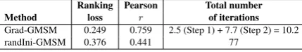
As opposed to the experimental scheme of RBF-SVR, we apply our regular training proce-dure on SCL-OPP lexicon. We consider it im-portant that the learned model generalizes well to phrases of variable length, hence we consider the training of one model per phrase length not con-ducive. Rather, we argue that training CMSM can and should be done independent of the length of phrases, by ultimately using the combination of different length phrases for training and testing. Also, our approach does not use information ex-tracted from other resources (such as Word2vec) nor POS tagging, i.e., we perform a light-weight training with fewer features. Still, we were able to obtain Pearsonr= 0.759in the task of regression. Table5presents the results obtained by random initialization in CMSM and Grad-GMSM on the SCL-OPP dataset. In both methods we apply early
stopping and perform ten-fold cross-validation. In Grad-GMSM, the total number of iterations again includes the iterations in both learning phases, and still it shows a faster convergence toward mini-mum ranking loss.
Ranking Pearson Total number
Method loss r of iterations
[image:7.595.310.525.144.181.2]Grad-GMSM 0.249 0.759 2.5 (Step 1) + 7.7 (Step 2) = 10.2 randIni-GMSM 0.376 0.441 77
Table 5: Performance comparison for different ini-tializations in SCL-OPP
Finally, we repeated the experiments on the Grad-GMSM model with values ofm, i.e., differ-ent numbers of dimensions. For each dimension number, we took the average of5runs. As shown in Table6, the results do improve only marginally when increasingmover several orders of magni-tude. Also the number of required iterations re-mains essentially the same, except for m = 1, which does not exploit the matrix properties. We see that – as opposed to vector space models – good performance can be achieved already with a very low number of dimensions.
Number of Ranking Pearson Total number
dimensions loss r of iterations
1 0.441 0.487 20.3
2 0.270 0.728 12.8
3 0.269 0.731 10.6
10 0.266 0.736 12.3
20 0.263 0.741 11.1
50 0.258 0.748 10.6
100 0.253 0.754 9.6
300 0.245 0.763 9.6
Table 6: Performance comparison for different di-mensions in SCL-OPP
5 Conclusion
perfor-mance of training CMSMs in sentiment prediction of phrases with opposing polarities and observed that the model captures compositionality well in such phrases. Since CMSMs turn out to be very robust against the choice of dimensionality, we conclude that choosing low-dimensional matrices as word representations lead to a reduced training time and still very good performance. In the fu-ture, we plan to extensively compare the learning of word matrix representations with vector space models in the task of sentiment analysis on several datasets.
References
Ameeta Agrawal and Aijun An. 2014. Kea: Sentiment analysis of phrases within short texts. In Preslav Nakov and Torsten Zesch, editors, Proceedings of the 8th International Workshop on Semantic Evalu-ation (SemEval 2014). pages 380–384.
Gottlob Frege. 1884. Die Grundlagen der Arithmetik: eine logisch-mathematische Untersuchung über den Begriff der Zahl. Breslau, Germany: W. Koebner. James Hong and Michael Fang. 2015. Sentiment
anal-ysis with deeply learned distributed representations of variable length texts. Technical report, Stanford University.
Svetlana Kiritchenko and Saif M Mohammad. 2016a. The effect of negators, modals, and degree adverbs on sentiment composition. In Alexandra Balahur, Erik van der Goot, Piek Vossen, and Andrés Mon-toyo, editors, Proceedings of the 7th Workshop on Computational Approaches to Subjectivity, Senti-ment and Social Media Analysis (WASSA). pages 43–52.
Svetlana Kiritchenko and Saif M Mohammad. 2016b. Sentiment composition of words with opposing po-larities. In Kevin Knight, Ani Nenkova, and Owen Rambow, editors, Proceedings of North American Chapter of the Association for Computational Lin-guistics: Human Language Technologies (NAACL-HLT 2016). pages 1102–1108.
Jean Maillard and Stephen Clark. 2015. Learning adjective meanings with a tensor-based skip-gram model. In Afra Alishahi and Alessandro Mos-chitti, editors, Proceedings of the Nineteenth Con-ference on Computational Natural Language Learn-ing (CoNLL 2015). pages 327–331.
Tomas Mikolov, Kai Chen, Greg Corrado, and Jef-frey Dean. 2013a. Efficient estimation of word representations in vector space. arXiv preprint arXiv:1301.3781.
Tomas Mikolov, Ilya Sutskever, Kai Chen, Greg S Cor-rado, and Jeff Dean. 2013b. Distributed represen-tations of words and phrases and their composi-tionality. In Chris J.C. Burges, Léon Bottou, Max
Welling, Zoubin Ghahramani, and Kilian Q. Wein-berger, editors,Advances in neural information pro-cessing systems (NIPS 2013). pages 3111–3119. Jeff Mitchell and Mirella Lapata. 2010. Composition
in distributional models of semantics.Cognitive sci-ence34(8):1388–1429.
Kaare B. Petersen and Michael S. Pedersen. 2012.The Matrix Cookbook. Technical University of Den-mark. Version 20121115.
Sebastian Rudolph and Eugenie Giesbrecht. 2010. Compositional matrix-space models of language. In Jan Hajic, Sandra Carberry, and Stephen Clark, ed-itors, Proceedings of the 48th Annual Meeting of the Association for Computational Linguistics (ACL 2010). pages 907–916.
Richard Socher, Brody Huval, Christopher D Man-ning, and Andrew Y Ng. 2012. Semantic composi-tionality through recursive matrix-vector spaces. In Jun’ichi Tsujii, James Henderson, and Marius Pasca, editors,Proceedings of the 2012 Joint Conference on Empirical Methods in Natural Language Process-ing and Computational Natural Language LearnProcess-ing (EMNLP-CoNLL 2012). pages 1201–1211.
Richard Socher, Alex Perelygin, Jean Y Wu, Jason Chuang, Christopher D Manning, Andrew Y Ng, and Christopher Potts. 2013. Recursive deep models for semantic compositionality over a sentiment tree-bank. InProceedings of the conference on empirical methods in natural language processing (EMNLP 2013). pages 1631–1642.
Aditya Timmaraju and Vikesh Khanna. 2015. Senti-ment analysis on movie reviews using recursive and recurrent neural network architectures. Semantic Scholar.
Xingyou Wang, Weijie Jiang, and Zhiyong Luo. 2016. Combination of convolutional and recurrent neural network for sentiment analysis of short texts. In Yuji Matsumoto and Rashmi Prasad, editors, Pro-ceedings of the 26th International Conference on Computational Linguistics (COLING 2016). pages 2428–2437.