Theoretical Formulation and Analysis of the
Deterministic Dendritic Cell Algorithm
Feng Gua, Julie Greensmith and Uwe Aickelinb aSchool of Computing, University of Leeds, LS2 9JT, UK bSchool of Computer Science, University of Nottingham, NG8 1BB, UK
Abstract
As one of the emerging algorithms in the field of Artificial Immune Systems (AIS), the Dendritic Cell Algorithm (DCA) has been successfully applied to a number of challenging real-world problems. However, one criticism is the lack of a formal definition, which could result in ambiguity for understand-ing the algorithm. Moreover, previous investigations have mainly focused on its empirical aspects. Therefore, it is necessary to provide a formal def-inition of the algorithm, as well as to perform runtime analyses to reveal its theoretical aspects. In this paper, we define the deterministic version of the DCA, named the dDCA, using set theory and mathematical functions. Runtime analyses of the standard algorithm and the one with additional segmentation are performed. Our analysis suggests that the standard dDCA has a runtime complexity ofO(n2) for the worst-case scenario, wherenis the number of input data instances. The introduction of segmentation changes the algorithm’s worst case runtime complexity to O(max(nN, nz)), for DC population sizeN with size of each segmentz. Finally, two runtime variables of the algorithm are formulated based on the input data, to understand its runtime behaviour as guidelines for further development.
Key words: Artificial Immune Systems, Dendritic Cell Algorithm, Runtime Analysis, Formulation and Formalisation
1. Introduction
system from which AIS draw inspiration, is evolved to protect the host from a wealth of invading micro-organisms. AIS are developed to provide similar defensive properties within a computing context. Initially, AIS were based on simple models of the human immune system. As noted by Stibor et al. [29], ‘first generation’ immune algorithms, such as negative selection and clonal selection, do not produce the same high-quality performance as the human immune system. These algorithms, negative selection in particular, are prone to problems with scalability and the generation of excessive false alarms, when used to solve problems such as network-based intrusion de-tection. Recent AIS use more rigorous and up-to-date immunology and are developed in collaboration with modellers and immunologists. The resulting algorithms are believed to encapsulate the desirable properties of immune systems, including robustness, error tolerance, and self-organisation [7].
One such ‘second generation’ immune algorithms is the Dendritic Cell Al-gorithm (DCA) [10]. The alAl-gorithm is inspired by functions of the dendritic cells (DCs) of the innate immune system, while incorporating principles of a key novel theory in immunology, named the danger theory [21]. An abstract model of natural DC behaviour is used as the foundation of the developed algorithm. The DCA has been successfully applied to numerous security-related problems, including port scan detection [10], botnet detection [1] and as a classifier for robot security [25]. These applications refer to the area of anomaly detection, which is essentially one particular type of binary classifi-cation with an ‘anomalous’ class and a ‘normal’ class. According to results of these applications, the DCA has shown not only good performance in terms of detection rate, but also the ability to reduce the rate of false alarms in comparison to other systems, such as Self Organising Maps (SOM) [13].
the algorithm in a clear and accessible manner.
Previous investigations have mainly focused on its empirical aspects, ev-idenced by experimental results on a range of problem domains. Except for the geometry analysis of Stibor et al. [28] that was later extended in Oates’s thesis [24], theoretical analysis of the DCA has barely been per-formed, and most theoretical aspects of the algorithm have not yet been revealed. Other immune inspired algorithms, such as negative and clonal selection algorithms, were theoretically presented in [30]. Elberfeld and Tex-tor [9] theoretically analysed string-based negative selection algorithms, to show the possibility of reducing the worst-case runtime complexity from ex-ponential to polynomial, through compressing detectors. More recently, the work of Zarges [31, 32] theoretically analysed one of the vital components of the clonal selection based algorithms, namely inversely proportional muta-tion rates. Jansen and Zarges [19] performed a theoretical analysis of immune inspired somatic contiguous hypermutations for function optimisation. As a result, it is important to conduct a similar theoretical analysis of the DCA, to determine its runtime complexity and numerous other algorithmic properties, in line with other AIS.
2. The Dendritic Cell Algorithm
2.1. Biological Background
The DCA is inspired by functions of the dendritic cells (DCs) of the innate immune system, which forms part of the body’s first line of defence against invaders. DCs exhibit the ability to combine a multitude of molecular in-formation and to interpret this inin-formation for the T-cells of the adaptive immune system. This could lead to the induction of various immune re-sponses against perceived pathogenic threats. Therefore, DCs are often seen as detectors responsible for policing different tissues, as well as inductive mediators for a variety of immune responses.
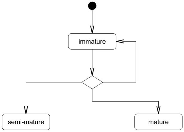
In general, two types of molecular information are processed by DCs, namely ‘signal’ and ‘antigen’. Signals are collected by DCs from their local environment and consist of indicators of the health status of the monitored tissue. Throughout its lifespan, an individual DC will exist in one of three states, namely ‘immature’, ‘semi-mature’ and fully ‘mature’, as shown in Figure 1. In the initial immature state, DCs are exposed to a combination of signals, and perform phagocytosis to ingest substances from their surround-ings. Based on the concentration of presented signals, DCs differentiate into either a ‘fully mature’ form to activate the adaptive immune system, or a ‘semi-mature’ form to suppress it. If a DC is exposed to a combination of signals generated from a healthy or steady state tissue environment, such as no occurrence of tissue damage, it more likely becomes a semi-mature DC. Conversely, if a DC is presented with a combination of signals generated from a damaged tissue environment, such as the presence of unregulated cell death, it more likely differentiates into a fully mature DC. Natural DCs bind to and process many cytokine signals. In an abstract model of DC behaviour developed by Greensmith [10], the following categories are defined.
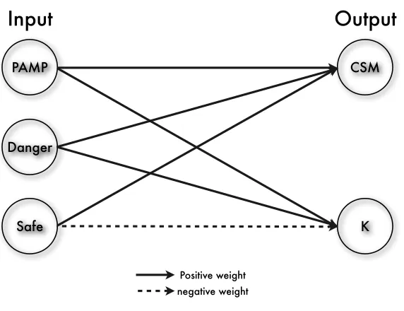
• PAMP: Pathogenetic Associated Molecular Patterns, molecular signa-tures of pathogens which are recognised by Toll-Like Receptors (TLRs) on the surface of DCs, and they are highly influential to the transition from immature state to fully mature state;
[image:5.612.150.458.129.351.2]
Figure 1: A state-chart describing the three states of an individual DC.
• Safe signals are derived from the cells that encounter apoptosis (pro-grammed cells death), TNF-α (Tumour Necrosis Factor) is one candi-date of safe signals, they contribute to the maturation from immature state to semi-mature state;
During the immature state, DCs also collect debris in the tissues which are subsequently combined with the environmental signals. Some of the ‘sus-picious’ debris collected are known as antigens, and they are proteins origi-nating from potential invading entities. DCs combine the ‘suspect’ antigens with evidence in the form of signals to correctly instruct the adaptive im-mune system to respond, or become tolerant to the presented antigens. For more detailed information regarding the underlying biological mechanisms, please refer to [10, 21].
2.2. Algorithmic Details
natural system, there are two types of input data, namely ‘antigen’ and ‘sig-nal’. It is generally assumed that certain causal relationship exists between the two data streams. Antigens are categorical values that can be various states of a problem domain or the entities of interest associated with a moni-tored system. Signals are represented as vectors of real-valued numbers, and they are measures of a monitored system’s status within certain time periods. In real-world applications, antigens represent what is to be classified within a given problem domain. For instance, they can be process IDs in com-puter security problems [1, 11], a small range of positions and orientations of robots [25], the proximity sensors of online robotic systems [22], or the time stamps of records collected in biometric data [17]. Signals represent system context of a host or a measure of network traffic [1, 11], the readings of var-ious sensors in robotic systems [25, 22], or the biometric data captured from a monitored automobile driver [17]. Signals are normally pre-categorised as ‘PAMP’,‘Danger’ or ‘Safe’. The semantics of these signal categories is listed as follows:
• PAMP: increases in value as the observation of anomalous behaviour, it is a confidence indicator of anomaly, which usually is presented as signatures of the events that can definitely cause damage to the system; • Danger: reflects to potential anomalies, as the values increases, the confidence of the abnormal status of the monitored system increases accordingly;
• Safe: increases in value in conjunction with observed normal behaviour, this is a confidence indicator of normal, predictable or steady-state sys-tem behaviour.
PAMP
Danger
Safe K
CSM
Input
Output
Positive weight negative weight
[image:7.612.165.451.125.345.2]Wednesday, 11 April 12
Figure 2: An illustration of the signal transformation process of the DCA.
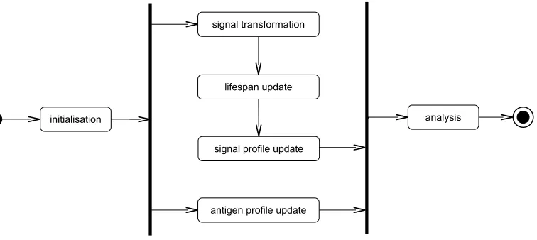
In order to achieve its detection ability, the DCA initialises a popula-tion of artificial DCs operating in parallel as detectors. Each DC is given a distinct limit of its lifespan, which creates a dynamic time window effect in the population [26]. This leads to the same signal and antigen data streams being processed by every DC, during different time periods across the anal-ysed time series. A temporal correlation between signals and antigens is also performed by each DC internally, to capture the causal relationship within the data. As suggested in [12], to perform correct correlation, the signals are supposed to appear after the antigens, and the delay should be shorter than the time window created by each DC.
[image:8.612.121.499.128.297.2]
Figure 3: An illustration of different steps of the DCA, where the initialisation and analysis steps are performed at the population level and the rest of the steps (bounded within the two vertical lines) are performed at the individual DC level.
mality indicated by its tendency toward −∞ or +∞. As soon as the DC’s lifespan reaches zero, it stops performing signal transformation and temporal correlation. The association between the cumulativeKand sampled antigens within the DC, termed ‘processed information’, is then accumulated by the analysis phase to produce the final detection results. Once a matured DC has presented the processed information, it is reset to its default form. Here, the population size is generally kept constant, but can be user specified. The entire process of different steps of the DCA is illustrated in Figure 3.
3. Formalisation of the DCA
3.1. Data Structures
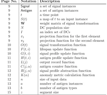
Define Signal ⊆ Rm and Antigen ⊆
N as the two types of input data.
Within a discrete time space Time = {1,2, . . . , t, . . .}, the input data can be defined as a function S : Time → Signal∪ Antigen, and S(t) is a data instance at a time point t ∈ Time. Elements from Signal are input signal instances of the algorithm, and are represented as m-dimensional real-valued vectors. These are usually normalised into a non-negative range, e.g. [0,1], as the input to the DCA. In many applications, m = 3 is the standard case, corresponding to the three input signal categories of the DCA as described in Section 2. Elements fromAntigenare categorical identifiers of certain objects to be classified, and are often represented as natural numbers starting from one, where the order is ignored.
Define the weight matrix of signal transformation as
W=
w11 · · · w1m w21 · · · w2m
where each entry wij ∈ R. The weight matrix W is used to transform the m-dimensional input signals to two categories of output signals, namely ‘CSM’ and ‘K’. It is usually predefined by users and kept constant during runtime. Entries in the weight matrix are based on empirical results from the underlying immunology of natural DCs [10].
Let Population be an index set of DCs and N = |Population| be the population size (N = 100 is a popular choice). The index of a DC is i ∈ Population. The function of assigning the initial lifespan to a DC is defined as I : Population → R, where I(i) 6= I(j) (i 6= j ∈ Population). The function of initialising the antigen profile of the DC is defined as M :
Population →(ai1, ai2, ..., aik, ...), where (ai1, ai2, ..., aik, ...) is a sequence stor-ing the antigen instances sampled by a DC and aik ∈ Antigen. The initial signal profile of a DC is usually set to zero.
The output of each DC is stored as a pair (aik, ri) ∈ Antigen×R in a list, where ri is the signal profile of a DC when it reaches a termination condition. We also define π1 and π2 as projection functions to obtain the first and second elements of a pair respectively.
3.2. Procedural Operations
the algorithm’s runtime analysis. At the beginning (t= 1), the algorithm ini-tialises all the DCs indexed byPopulation, through assigning the initial values of lifespans and signal profiles, named ‘DC initialisation’. The value ofI(i) depends on the distribution function used to generate the initial lifespans of DCs. Both uniform distribution and Gaussian distribution can be applied to generate I(i). The antigen profile of each DC is set as Null or empty, while the signal profile is set as zero.
Definition 1 (signal transformation). The signal transformation function
O :Time→R×R is defined as
O(t) =
WTS(t), if S(t)∈Signal; 0, otherwise.
This operation is executed whenever S(t) ∈ Signal holds, and it performs the multiplication between a transposed 2×m matrix and anm-dimensional vector to produce a two dimensional vector of output signals, ‘CSM’ and ‘K’. These are related to when and how to make decisions respectively. In the case that S(t)∈Antigen, the function returns a zero vector.
Definition 2 (lifespan update). The lifespan update function F :Time×
Population →R is defined as
F(t, i) =
I(i), if t= 1;
I(i)−π1(O(t)), if F(t−1, i)≤0; F(t−1, i)−π1(O(t)), otherwise.
When t = 1, the initial value of F isI(i), which is the initial lifespan of the DC with an index i. It is repeatedly subtracted by CSM signal until the termination condition, F(t−1, i)≤0, is reached. The function is then reset to ‘I(i)−π1(O(t))’ (notI(i)), due to the function O(t) being executed at a regular basis, e.g. at every single time point t.
Definition 3 (signal profile update). The signal profile update function
G:Time×Population→R is defined as
G(t, i) =
0, if t= 1;
π2(O(t)), if F(t−1, i)≤0; G(t−1, i) +π2(O(t)), otherwise.
termination condition is reached. The function is then reset to ‘π2(O(t))’ (not 0), due to the function O(t) being executed at a regular basis, e.g. at every single time point t ∈Time.
Definition 4 (antigen profile update). The antigen profile update func-tion H :Time×Population→(ai1, ai2, . . . , aik, . . .) is defined as
H(t, i) =
∅, t= 1;
(H(t−1, i), S(t)), if S(t)∈Antigen and t >1; H(t−1, i) if S(t)∈Signal and t >1,
whereHis initially empty. As a new antigen instance arrives, it is sampled by the DC with an indexiand its antigen profile is updated until the termination condition is reached. This function merely appends a list to another, which can be done in constant time regardless of the length of the lists, and thus considered as one-step operation as well. It is performed individually by each DC and the index of the DC selected to sample an incoming S(t)∈Antigen
is defined as i ≡ θ mod N (i is congruent with θ modulo N), where θ is the number of antigen instances up to time t. This is termed the ‘sequential sampling’ rule.
Definition 5 (output record). Let ri =G(t, i) s.t. F(t−1, i)≤ 0 be the signal profile of a DC, and L : N → Antigen×R denote the function that maps an index j ∈ N to an element of the output list. The output record function is defined as
L(j) = (aik, ri) ∀k
where L(j) is the jth element of the list. The antigen profile often consists of multiple values while the signal profile only contains one single value in the DC with an indexi. This function essentially enumerates all the possible pairs and appends them to the output list, where each of them is assigned an index j. The list is then used to produce the final detection results in the analysis phase of the DCA.
Definition 6 (antigen counter). The antigen counter function C : N×
Antigen→ {0,1} is defined as
C(j, α) =
Definition 7 (signal profile abstraction). The signal profile abstraction function R :N×Antigen→R is defined as
R(j, α) =
π2(L(j)), if π1(L(j)) =α; 0, otherwise.
In the two functions above, α∈Antigen is an antigen type. The function C is used to count the number of instances of antigen type α, and the function R is used to calculate the sum of all K values associated with antigen type α. These two operations are performed for every antigen type and involve scanning the sequence of L(j) in its entirety.
Definition 8 (anomaly metric calculation). Given the number of input instances is equal to n, the anomaly metric calculation function is defined as.
K(α) = γ
β with β = n
X
j=1
C(j, α) and γ = n
X
j=1
R(j, α)
As Antigen6=∅ and α∈Antigen, the minimum number of antigen instances is equal to one, so is the minimum number of antigen types. Therefore, we have β ≥ 1. A threshold ε can be applied for further classification. The value of the threshold depends on the underlying characteristics of the dataset used. An antigen type α is classified as anomalous ifK(α)> ε, and normal otherwise.
4. Analysis of Runtime Complexity
4.1. The Standard DCA
As mentioned previously, applications of the DCA are referred to the area of anomaly detection. In AIS, one popular anomaly detection algo-rithm is known as the negative selection algoalgo-rithm, which was shown to have an exponential runtime complexity [30]. An attempt of reducing the worst-case runtime complexity from exponential to polynomial was reported in [9], however this reduction is only applicable when the input feature space is bit strings instead of real numbers. Other popular anomaly detection al-gorithms are more or less derived from techniques in machine learning [4], e.g. K-Nearest Neighbour (KNN) with a runtime complexity of O(nd) [8], decision trees algorithms with an exponential runtime complexity [8], and support vector machines (SVM) with a runtime complexity of O(n2d) [3], where n is the number of input instances and d is the dimensionality. As a result, the subsequent runtime analysis of the DCA reveals if the algorithm is competitive against other state-of-the-art anomaly detection algorithms.
Let a be the number of antigen instances within the input data, b = |Antigen| be the number of antigen types and N be the size of the DC pop-ulation. According to previous applications [1, 25, 11, 22, 17], N is usually user defined and independent of the increase of data size n. However, we often assume that 1≤N ≤n. In order to make the following analyses more general, the population size N is considered a parameter of the algorithm. As the type of input data instances is either AntigenorSignal, if the number of antigen instances is equal to a, the number of signal instance isn−a. For the ease of analysis, the algorithm is divided into three phases as follows:
1. Initialisation phase - Line 1 to Line 3; 2. Detection phase - Line 4 to Line 19; 3. Analysis phase - Line 20 to Line 26.
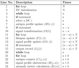
The calculation of runtime is performed phase by phase. LetT1(n),T2(n) and T3(n) be the runtime of each phase respectively, and T(n) = T1(n) + T2(n) + T3(n) is the overall runtime of the algorithm. Details of all the primitive operations of the algorithm are listed in Table 1, including theline number and the description of each operation as well as the number of times an operation is executed, corresponding to Algorithm 1.
follows.
T1(n) = N+N =O(N)
The runtime of the detection phase depends on the data size n, the number of antigen instances a, the number of signal instancesn−a and the size of the DC population N. Thus the runtime of the detection phase is calculated as follows.
T2(n) = n+ 3a+ 2(n−a) + 5(n−a)N = 3n+ 5N(n−a) +a ⇒ {a ≤n}
T2(n) = O(n) +O(N(n−a)) +O(a) = O(nN)
The runtime of theanalysis phaseis dependent on the size of the output list that is equal to the number of antigen instances a and the number of antigen types b. The value of b is determined by the number of states or entities to classify within a problem domain. Here we merely focus on the worst-case scenario, which occurs ifb=a, and the number of antigen types is equal to the number of antigen instances. Therefore, we have 1≤b ≤a≤n. The runtime of the analysis phase is thus calculated as follows.
T3(n) =a+ab+ 3ab=O(n2)
Theorem 1. The runtime complexity of the standard DCA is bounded by
O(n2), with respect to the data size n.
Proof.
T(n) = T1(n) +T2(n) +T3(n)
⇒ {T1(n) =O(N), T2(n) = O(nN), and T3(n) = O(n2)} T(n) = O(N) +O(nN) +O(n2)
⇒ {1≤N ≤n} T(n) = O(n2)
Bounds provided by O-notation are asymptotically tight.
algorithms. According to previous applications [1, 11, 25, 22, 17, 14], we often have N n. Such a premise makes the runtime complexity of algo-rithm’s initialisation and detection phases overall linear, while the analysis phase stays quadratic. This leads to the following work of modifying the analysis phase of the algorithm via an introduction of segmentation.
4.2. The DCA with Segmentation
Segmentation is introduced to adapt the algorithm to online analysis [16]. Instead of analysing the processed information in a single operation at the termination of the detection phase, the output list is partitioned into smaller segments and the analysis is performed within each segment. We postulate that segmentation could potentially generate finer grained results, as well as performing analysis in parallel with the detection process. Here, we focus on the antigen based segmentation approach, as it is more favourable in actual applications [16]. One may think that the system with segmentation produces the final detection results much faster, as the analysis is performed during detection on a much smaller chunk of processed information. Based on the analysis of the standard DCA, it is possible to theoretically analyse the effect of segmentation on the algorithm’s runtime complexity. Let z be a predefined segment size and 1≤z ≤n. A segment is generated once the size of the output list reachesz, and an analysis on the current batch of processed information in the output list is performed.
As a post-processing mechanism, segmentation only affects theanalysis phase of the algorithm, but not the initialisation phase or detection phase. The search space of the analysis of a segment is determined by the value of z. The number of segments created is equal to dn/ze, and they are indexed by {1,2, . . . , k, . . . ,dn/ze}. Let ak ≤ z and bk ≤ z denote the number antigen instances and the number of antigen types in thekth segment respectively. As a result, the runtime complexity of each segment at the analysis phase is Tk
3(n) =akbk ≤z2 =O(z2).
Theorem 2. The runtime complexity of the DCA with segmentation is bounded by O(max(nN, nz)), with respect to the data size n, the DC population size
Proof.
⇒ {T1(n) =O(N) and T2(n) = O(nN)}
T(n) = O(N) +O(nN) +
dn/ze
X
k=1
akbk ≤ O(N) +O(nN) +dn/zeO(z2)
⇒ {1≤N ≤n and 1≤z ≤n}
T(n) = O(N) +O(nN) +O(nz) =O(max(nN, nz))
As shown in Theorem 2, the introduction of segmentation changes the overall runtime complexity of the algorithm to O(max(nN, nz)). Depending on the values of N and z, the runtime complexity can be either quadratic (N =n∨z =n) or linear (N n∧z n). This is very attractive for online detection tasks, as it provides a means of online analysis that continuously and periodically produces results during detection. Additionally, the DCA with segmentation produces significantly different and better results than the standard version [16]. Therefore, segmentation is an important and necessary addition to the DCA from a practical point of view. Thus far only static segmentation with a fixed segment size has been applied to the DCA. The effect of variable segment sizes on the detection performance still requires further investigation.
5. Formulation of Runtime Properties
5.1. Number of Matured DCs
The number of matured DCs within a time interval is related to the reset frequency of the DC population, which indicates the work-load of the DC population. This can be used to determine whether the current setup of the current system should be altered. If the frequency of DC resetting is too high, most of the DCs become matured and get reset before they acquire a sufficient amount of information. As a result, the range of lifespans of the DC population should be extended, allowing more information to be obtained. In conduction with extending the range of lifespans of the DC population, it is necessary to also increase the size of the DC population, so that the lifespans do not become sparse.
This becomes crucial if the system is deployed online, as an online system is often required to perform continuous detection and adapt to the changes of real-time situations. The number of matured DCs in the DC population depends on the distribution function used for the generation of DC lifespans, in addition to the input data within the time interval of interest. To make the analysis manageable, two types of distributions for generating the initial DC lifespans are considered, namely uniform distribution [2] and Gaussian distribution [2]. The calculations will be done through using the mean value of lifespans of the DC population and the mean value of CSM signals cor-responding to all the input signal instances. They focus on the average number of matured DCs within a given time interval rather than the partic-ular number per iteration. However, as the time interval is reduced, e.g. to the duration of one iteration, the two numbers could become approximate to each other.
Proposition 1 (uniform distribution). If the lifespans of the DC population are generated from an arithmetic series xi = x1 + (i − 1)d, where xi is
the nth element, x1 is the first element and d is the interval between two successive elements, the number of matured DCs in the DC population δ can be calculated as follows.
δ=
$
NPte
t=tbπ1(O(t))
(te−tb)(x1+N2−1d)
%
is equal to N, the lifespan of the last DC with an index i = N is given as xN =x1+(N−1)d. As demonstrated in Section 3, the termination condition where a DC matures as soon as its lifespan reaches zero through subtracting the CSM signals.
Proof.
⇒ {ϕ=
Pte
t=tbπ1(O(t))
te−tb
and µ1 = x1+xN
2 =x1+
N −1 2 d}
δ =
N ϕ µ1
=
$
NPte
t=tbπ1(O(t))
(te−tb)(x1+ N2−1d)
%
Where ϕis the mean value of theCSMsignals within the interval [tb, te] and µ1 is the mean lifespan of the DC population.
Uniform distribution is used in the dDCA [12] to generate the initial lifes-pans of the DC population. This produces a set of values that are uniformly distributed within a certain range. According to Proposition 1, if the param-eters (first element x1 and the interval d) of the arithmetic series are given, the number of matured DCs within the time interval [tb, te] can be calculated accordingly.
Proposition 2 (Gaussian distribution). If the lifespans of the DC population are generated from a Gaussian distribution x∼ N(µ, σ2), then the following formula holds.
Pr
$
NPte
t=tbπ1(O(t))
(µ−√2σ
N)(te−tb)
%
≤δ ≤
$
NPte
t=tbπ1(O(t))
(µ+√2σ
N)(te−tb)
%!
Proof.
⇒ {ϕ=
Pte
t=tbπ1(O(t))
te−tb
and µ2 ∼ N(µ, σ2 N)} Pr
µ−2√σ
N ≤µ2 ≤µ+ 2 σ √
N
= 0.95
⇒ {δ=
N ϕ µ2 = $ N µ2(te−tb)
te X t=tb π1(O(t)) % } $
NPte
t=tbπ1(O(t))
(µ− √2σ
N)(te−tb)
%
≤δ≤
$
NPte
t=tbπ1(O(t))
(µ+√2σ
N)(te−tb)
%
Pr(·) is the probability operator. If the sample size is N, the sample mean µ2 is bounded by a Gaussian distribution x ∼ N(µ,σ
2
N) [2]. The lower and upper bounds of the sample mean can be used to induce the bounds of the number of matured DCs.
In practice, Gaussian distribution has not been used for generating the lifespans of the DC population, but it has been of great interest [27] and would be a priority of future investigation. According to Proposition 2, if we know the mean (µ) and variance (σ2) of the Gaussian distribution from which the lifespans of the DC population are generated, the size of DC population N, and the input data instances within the time interval [tb, te], we can show that there is a 0.95 chance the number of matured DCs is bounded by the lower and upper bounds. This could provide sufficient information for adjusting the system according to real-time scenarios.
5.2. Number of Processed Antigens
we focus on formulating the relationship between the number of processed antigens and the input data, in particular, the number of input antigens. Let θ ∈ N at t ∈ Time be the number of input antigens that are fed into the system, and δ be the mean lifespan of the DC population. Similar to Proposition 1 or Proposition 2, the calculations focus on the average number of processed antigens within a given time interval rather than the particular duration per iteration. As the time interval decreases, e.g. to the duration of one iteration, the two numbers could also be approximate to each other.
The method of calculating the number of processed antigens within a given time interval [tb, te] should be introduced first. It is similar to placing balls into a number of bins that are ordered based on their indexes in a sequential manner. Placing starts from the first bin then the second bin and so forth. If we reach the last bin, the process starts over again. In the end, a number of bins, starting from the first one, are taken and the number of balls contained is counted. The balls are equivalent to input antigens, the bins are equivalent to DCs, and the action of counting the number of balls is equivalent to the action of counting the number of processed antigens. Proposition 3 formulates the relationship between the number of processed antigens and the input data in two cases.
Proposition 3 (number of processed antigens). Let ν be the number of processed antigens within a given interval [tb, te], c ≡ δ mod N and d ≡ θ mod N, the following formula of ν holds.
ν =
δ−Nδ
N
)(1 +θ
N
, if c < d; δ−N −Nδ
N θ N
Proof.
{transform modulus to floor functions}
⇒ c=δ−N
δ N
and d=θ−N
θ N
⇒ {sequential sampling} Case 1 :c < d
ν =c
θ N
+c=
δ−N
δ
N 1 +
θ N
Case 2 :c≥d
ν =c
θ N
+d=
δ−N−N
δ N θ N +θ
The number of antigens sampled by each DC is determined byθ modN, but as only matured DCs present processed antigens, the number of processed antigens is determined by δ and the maximum of cand d.
The formulas for the number of processed antigens have two cases, de-pending on the relationship between c ≡ δ mod N and d ≡ θ modN. These formulas can relate the runtime variables of the algorithm to the in-put data, without actually running the algorithm. This provides theoretical insights into tuning the algorithm for a given problem.
6. Conclusions and Future Work
Moreover, two runtime variables are formulated, the number of matured DCs and the number of processed antigens. This shows how the algorithm behaves within a given time interval based on the input data without actually running the algorithm. As a result, the formulas of two runtime variables can be used as the indicators of adjusting the setup of the system according to real-time situations during detection. This an important step for under-standing some of the potentially beneficial properties of the algorithm from a theoretical perspective, which could facilitate further investigations on the usefulness of these properties with respect to anomaly detection problems.
This work gives application independent insights to the algorithm, which can be used as guidelines for future development. One of the goals of fu-ture development of the DCA is to turn it into an automated and adaptive online detection system, and such a system has certain requirements to ful-fil. Firstly, the system has to be computationally efficient. The analysis of the runtime complexity of the DCA shows even in worst case scenarios its runtime complexity is competitive against other popular anomaly detection algorithms. Secondly, the system should be able to adapt to real-time sce-narios encountered during detection. This requires the insights of how the algorithm behaves during runtime, which can be assessed from the two run-time variables. As a result, new components can be developed and integrated within the algorithm to adjust the system based on the assessment of these two runtime variables.
In terms of future work, the specifications can be further simplified and the algorithm can be presented using functional programming approach [6], to reveal more algorithmic details. In addition, synthetic datasets generated from various probability density functions can be used to test the formu-las defined in this paper. We can also investigate other properties of the algorithm, for example, the moving window effect created by each DC and the relationship between the size of DC population and the detection per-formance. Different methods of generating the initial lifespans of the DC population should also be investigated, in addition to the relationship be-tween the weight matrix and the detection performance.
References
[2] A. C. Atkinson, M. Riani, and A. Cerioli. Exploring Multivariate Data with the Forward Search. Springer Series in Statistics. Springer, 2004. [3] C. J. C. Buerges. A Tutorial on Support Vector Mahinces for Pattern
Recognition. Data Mining and Knowledge Discovery, 2:121–167, 1998.
[4] V. Chandola, A. Banerjee, and V. Kumar. Anomaly detection: A survey.
ACM Computing Surveys (CSUR), 41(3):Article 15, 2009.
[5] T. H. Cormen, C. E. Leiserson, R. L. Rivest, and C. Stein. Introduction to Algorithms, Third Edition (Hardcover). The MIT Electrical Engi-neering and Computer Sicence Series. The MIT Press, 2009.
[6] G. Cousineau, M. Mauny, and K. Callaway. The Functional Approach to Programming. Cambridge University Press, 1998.
[7] L. N. de Castro and J. Timmis. Artificial Immune Systems: A New Computational Intelligent Approach. Springer-Verlag, 2002.
[8] R. O. Duda, P. E. Hart, and D. G. Stork. Pattern Classification. Wiley-Blackwell, 2nd edition, 2000.
[9] M. Elberfeld and J. Textor. Negative selection algorithms on strings with efficient training and linear-time classification. Theoretical Computer Sicence, 412(6):534–542, 2011.
[10] J. Greensmith. The Dendritic Cell Algorithm. PhD thesis, School of Computer Science, University of Nottingham, 2007.
[11] J. Greensmith and U. Aickelin. DCA for SYN Scan Detection. In
Proceedings of the Genetic and Evolutionary Computation Conference (GECCO), pages 49–56, 2007.
[12] J. Greensmith and U. Aickelin. The Deterministic Dendritic Cell Algo-rithm. In Proceedings of the 7th International Conference on Artificial Immune Systems (ICARIS), pages 291–303, 2008.
[13] J. Greensmith, J. Feyereisl, and U. Aickelin. The DCA: SOMe Compar-ison A comparative study between two biologically-inspired algorithms.
[14] F. Gu, J. Greensmith, and U. Aickelin. Further Exploration of the Dendritic Cell Algorithm: Antigen Multiplier and Time Windows. In
Proceedings of the 7th International Conference on Artificial Immune Systems (ICARIS), pages 142–153, 2008.
[15] F. Gu, J. Greensmith, and U. Aickelin. Exploration of the Dendritic Cell Algorithm with the Duration Calculus. InProceedings of the 8th In-ternational Conference on Artificial Immune Systems (ICARIS), pages 54–66, 2009.
[16] F. Gu, J. Greensmith, and U. Aickelin. Integrating Real-Time Anal-ysis With The Dendritic Cell Algorithm Through Segmentation. In
Proceedings of the Genetic and Evolutionary Computation Conference (GECCO), pages 1203–1210, 2009.
[17] F. Gu, J. Greensmith, R. Oates, and U. Aickelin. PCA 4 DCA: the application of Principal Component Analysis to the Dendritic Cell Al-gorithm. In Proceedings of the 9th Annual Workshop on Computational Intelligence (UKCI), 2009.
[18] E. Hart and J. Timmis. Application Areas of AIS: The Past, Present and the Future. Journal of Applied Soft Computing, 8(1):191–201, 2008.
[19] T. Janson and C. Zarges. Analyzing different variants of immune in-spired somatic contiguous hypermutations. Theoretical Computer Si-cence, 412(6):517–533, 2011.
[20] A. Jean-Raymond. The B-Book. Cambridge University Press, 1996.
[21] M. B. Lutz and G. Schuler. Immature, semi-mature and fully mature dendritic cells: which signals induce tolerance or immunity? TRENDS in Immunology, 23(9):445–449, 2002.
[22] M. Mokhtar, R. Bi, J. Timmis, and A. M. Tyrrell. A Modified Den-dritic Cell Algorithm for On-line Error Detection in Robotic Systems. InProceedings of the 11th IEEE Congress on Evolutionary Computation (CEC), pages 2055–2062, 2009.
[24] R. Oates. The Suitability of the Dendritic Cell Algorithm for Robotic Se-curity Applications. PhD thesis, School of Computer Science, University of Nottingham, 2010.
[25] R. Oates, J. Greensmith, U. Aickelin, J. Garibaldi, and G. Kendall. The Application of a Dendritic Cell Algorithm to a Robotic Classifier. InProceedings of the 6th International Conference on Artificial Immune (ICARIS), pages 204–215, 2007.
[26] R. Oates, G. Kendall, and J. Garibaldi. Frequency Analysis for Dendritic Cell Population Tuning: Decimating the Dendritic Cell. Evolutionary Intelligence, 1(2):145–157, 2008.
[27] R. Oates, G. Kendall, and J. Garibaldi. Classifying in the presence of uncertainty: a DCA persepctive. InProceedings of the 9th International Conference on Artificial Immune Systems (ICARIS), pages 75–87, 2010.
[28] T. Stibor, R. Oates, G. Kendall, and J. Garibaldi. Geometrical insights into the dendritic cell algorithm. InProceedings of the Genetic and Evo-lutionary Computation Conference (GECCO), pages 1275–1282, 2009.
[29] T. Stibor, J. Timmis, and E. Claudia. A Comparative Study of Real-Valued Negative Selection to Statistical Anomaly Detection Techniques. InProceedings of the 4th International Conference on Artificial Immune Systems (ICARIS), pages 262–375, 2005.
[30] J. Timmis, A. Home, T. Stibor, and E. Clark. Theoretical advances in artificial immune systems. Theoretical Computer Sicence, 403(1):11–32, 2008.
[31] C. Zarges. Rigorous runtime analysis of inversely fitness proportional muation rates. In Proceedings of Parallel Problem Solving from Nature (PPSN), pages 112–122, 2008.
Algorithm 1: Pseudocode of the DCA implementation, the selection of a DC when an antigen instance is presented is performed according to the ‘sequential sampling’ rule.
input : input data S(t) output: anomaly metric K(α)
1 foreach DC do /* Initialisation phase */
2 DC initialisation; 3 end
4 while input data do /* Detection phase */
5 if antigen then
6 select a DC i; 7 do H(t, i); 8 end
9 if signal then
10 do O(t);
11 foreach DC do
12 do F(t, i); 13 do G(t, i);
14 if F(t−1, i)≤0 then 15 do L(j);
16 end
17 end
18 end
19 end
20 while output list do /* Analysis phase */
21 foreach antigen type do 22 do C(j, α);
23 do R(j, α); 24 do K(α); 25 end
Line No. Description Times
1 for loop N
2 DC initialisation N
4 while loop n
5 ifstatement a
6 select a DCi a
7 antigen profile update (H(t, i)) a
9 ifstatement n−a
10 signal transformation (O(t)) n−a
11 for loop (n−a)×N
12 lifespan update (F(t, i)) (n−a)×N 13 signal profile update (G(t, i)) (n−a)×N
14 ifstatement (n−a)×N
15 output record (L(j)) (n−a)×N
20 while loop a
21 for loop a×b
[image:27.612.145.469.229.508.2]22 antigen counter (C(j, α)) a×b 23 signal profile abstraction (R(j, α)) a×b 24 anomaly metric calculation (K(α)) a×b
Page No. Notation Description
9 Signal a set of signal instances 9 Antigen a set of antigen instances
9 t a time point
9 S(t) a map oft to an input instance
9 W weight matrix of signal transformation
9 N DC population size
9 I an index set of DCs
9 π1 projection function for the first element 9 π2 projection function for the second element 10 O(t) signal transformation function
10 F(t, i) lifespan update function 10 G(t, i) signal profile update function 11 H(t, i) antigen profile update function 11 L(j) output record function
11 C(j, α) antigen counter function
12 R(j, α) signal profile abstraction function 12 K(α) anomaly metric calculation function
12 n size of input data
13 a number of antigen instances 13 b number of antigen types
[image:28.612.128.487.226.545.2]15 z segment size