Time domain wave separation using multiple microphones

Time domain wave separation using multiple microphones

Jonathan A. Kempa兲

School of Physics, University of Edinburgh, Room 4306, JCMB, Edinburgh EH9 3JZ, United Kingdom

Maarten van Walstijn

Sonic Arts Research Centre, Queen’s University Belfast, Room 1017, Belfast BT7 1NN, United Kingdom

D. Murray Campbell

School of Physics, University of Edinburgh, Room 7306, JCMB, Edinburgh EH9 3JZ, United Kingdom

John P. Chick

School of Engineering, University of Edinburgh, Room 4.114, Faraday Building, Edinburgh EH9 3JL, United Kingdom

Richard A. Smith

Smith Watkins Trumpets, Cornborough, Sheriff Hutton, Yorkshire YO60 6RU, United Kingdom

共Received 21 August 2009; revised 26 February 2010; accepted 12 March 2010兲

Methods of measuring the acoustic behavior of tubular systems can be broadly characterized as steady state measurements, where the measured signals are analyzed in terms of infinite duration sinusoids, and reflectometry measurements which exploit causality to separate the forward and backward going waves in a duct. This paper sets out a multiple microphone reflectometry technique which performs wave separation by using time domain convolution to track the forward and backward going waves in a cylindrical source tube. The current work uses two calibration runs共one for forward going waves and one for backward going waves兲to measure the time domain transfer functions for each pair of microphones. These time domain transfer functions encode the time delay, frequency dependent losses and microphone gain ratios for travel between microphones. This approach is applied to the measurement of wave separation, bore profile and input impedance. The work differs from existing frequency domain methods in that it combines the information of multiple microphones within a time domain algorithm, and differs from existing time domain methods in its inclusion of the effect of losses and gain ratios in intermicrophone transfer functions. ©2010 Acoustical Society of America. 关DOI: 10.1121/1.3392441兴

PACS number共s兲: 43.60.Pt, 43.58.Bh, 43.75.Fg 关AJZ兴 Pages: 195–205

I. INTRODUCTION

The acoustic behavior of tubular objects can be charac-terized by measuring the input impedance or input impulse

response using a loudspeaker and one or more

microphones.1,2These methods can usually be classified ei-ther as steady state methods which work by determining the frequency dependent acoustic impedance relative to test ob-jects of known impedance3or reflectometry methods which work by exploiting time domain windowing, for instance, by using a source tube which is long enough to allow direct separation of the waves in time at a single microphone.4–6 The major disadvantage of long source tubes is that acoustic losses become prohibitive at high frequencies, meaning that the bandwidth is limited; the major disadvantage of any two microphone method is that there are singularities when the intermicrophone distance matches integer multiples of half a wavelength. These singularities can be worked around by using more than two microphones.1–3

In this paper a new method is presented which uses mul-tiple microphones to keep track of overlapping forward and

backward going waves in a source tube. The technique relies on first measuring the time domain transfer function between every combination of two microphones and then exploiting causality to determine the forward and backward going waves at each microphone position in the time domain. Since calibration is based on measurements of the time domain transfer between microphones, no assumptions or prior knowledge are required of intermicrophone distances, the speed of sound or any acoustic propagation coefficients so long as they remain constant during the experiment. Once the backward and forward going waves in the tube are known, the impulse response can be calculated by deconvo-lution and this can be used to calculate the input impedance and bore profile.

This method can be applied to the measurement of a wide range of ducts including musical wind instruments and industrial pipe work. The input impedance can be used to determine the resonant frequencies, while bore reconstruc-tion can be used to spot imperfecreconstruc-tions in manufacture in addition to leaks, dents, and blockages that may appear over time. In industry often the precise internal dimension of an object are well known and in situtesting of components to spot the effects of corrosion before a leak occurs is useful. Comparative testing 共using one microphone without a full

a兲_{Author to whom correspondence should be addressed. Electronic mail:}

input impulse response measurement or bore reconstruction兲 has been used recently by Amiret al.7to find corrosion and blockages in heat exchangers in power stations. Using mul-tiple microphones clearly has benefits in terms of increasing the available information on a system. The proposed tech-nique converts the exactly determined two microphone prob-lem into an overdetermined multiple microphone probprob-lem, leading to an analysis which is more efficient at removing the effects of errors and noise.

II. TWO MICROPHONES

Various methods exist for analyzing the recordings at two microphones to calculate the impedance at a reference plane, as reviewed by Dalmont1 and Dickens et al.2 The complex frequency-dependent input impedance is related to the impulse response by a simple formula which means that methods designed to measure input impedance can also gen-erate the input impulse response and bore profile. Such meth-ods can be used to separate forward and backward going waves in time as long as the input impedance has already been measured accurately for all frequencies for the current test object. They do not allow direct separation of the for-ward and backfor-ward going waves in time for a new test ob-ject, however, without first remeasuring the input impedance for all frequencies. Measurement of the input impedance in-volves intrinsic singularities when the intermicrophone dis-tance matches half a wavelength. Multiple intermicrophone distances must therefore be used to obtain a successful wide-band result.3,8

Existing wave separation techniques, such as those de-signed by Piñero and Vergara,9 Seybert,10 and Guerard and Boutillon,11 have also been largely based on frequency do-main analysis and accurately known intermicrophone dis-tances. A recent time domain method by Nauclér et al.12 starts with the assumption that the sensors have identical frequency responses and zero losses for travel between the microphones. Wave separation is performed with any devia-tion from the above condidevia-tions being interpreted as being part of a measurement noise term. This method has proved to be resistant to the presence of white noise at the sensors in simulations but is yet to be applied to microphone based acoustic measurements where the nonidentical nature of the sensors are significant.

In order to combine more than two microphone mea-surements to reduce the effects of singularities when the wavelength obeys certain integer relationships with the inter-microphone distances, and to take advantage of causality, the method proposed here uses a novel time domain formulation with two calibrations to characterize the forward and back-ward going transfer between the microphones. The method is set out for two microphones before going on to generalize the method toM microphones.

III. APPARATUS

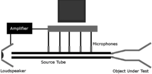
The apparatus consists of a brass source tube with an internal diameter of 9.7 mm, with Sennheiser KE4-211 mi-crophone capsules placed in the side wall and separated by distances of the order of 10 cm. A JBL 2426J compression

driver loudspeaker driven by a Denon hi-fi amplifier was coupled to one end of the tubes and an object under test placed at the other end. Sound input and output was handled with a Focusrite Saffire Pro 10 audio interface. A schematic of the apparatus is shown in Fig. 1.

The preferred method for impulse response measure-ment here is the logarithmic sine sweep technique, as the signal to noise ratio is very good for measurements lasting of the order of 10 s and the measurement quality is not com-promised by a moderate level of harmonic distortion in con-trast to maximum length sequence measurement.13 In this technique the excitation signal is deconvolved from the mea-surement to obtain a signal identical to that which we would have observed by putting in a pulse of one time sample du-ration but with a much better signal to noise ratio. It should be noted that, as it stands, the loudspeaker and microphone responses are still included in the system impulse response and further processing is necessary if we want to calibrate such effects out of the measurement. In practice signals can-not be produced and measured below around 20 Hz. This will limit the accuracy of the technique at low frequencies. The wavelength of a 20 Hz signal is approximately 17 m, however, and objects of practical interest for the current study will be significantly shorter than this, meaning that no resonances will be missed at low frequency. This means that the missing data points in calibration results can be estimated effectively by fitting a straight line to the absolute value and phase angle data in frequency domain.

The experiments that follow were carried out at a sample rate of 96 kHz, using a logarithmic sine sweep of length 221

samples played four times end to end. The signal was ramped in amplitude from maximal amplitude at 20 Hz, down to 0.1 of maximal amplitude at 500 Hz and then up to maximal amplitude again by the highest input frequency of 30 kHz in order to give a signal to noise ratio boost at low and high frequencies 共i.e., to maximize the bandwidth兲. An average of the signal during the second to fourth plays was then taken 共to give the periodic response to the periodic in-put兲. This was then divided in the frequency domain by the ramped excitation signal in order to obtain the system im-pulse response.

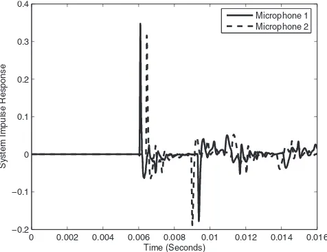
Figure 2 shows a plot of the system impulse response measured at two microphone positions with an intermicro-phone distance ofd= 12.5 cm where microphone 1 is closest to the loudspeaker. It is clear that a forward going impulse emitted from the loudspeaker arrives d/c⬇0.125/340

FIG. 1. Multiple microphone wave separation apparatus.

= 0.37 ms earlier at microphone 1 than at microphone 2. The complicated backward going reflections from an object placed on the end of the source tube are then received at microphone 2. They are received at microphone 1 after a time delay of 0.37 ms. It should be noted that the forward going wave has not entirely finished when the backward go-ing wave arrives, so the source tube is not long enough for conventional pulse reflectometry.

IV. FORWARD GOING TIME DOMAIN TRANSFER FUNCTION

The first requirement is to use acoustic measurement to characterize the transfer of sound between microphones. This can be achieved, in principle, by taking the system impulse response with a very long cylindrical calibration tube placed on the end of the source tube such that the waves in the source tube can be assumed to be only forward going. This requires that the cross-sectional area of the semi-infinite tube is the same as the source tube and that the calibration tube is sufficiently long that no measurable reflections return from it. The system impulse response at the first microphone can then be deconvolved from the system impulse response at the second microphone. In principle this may be done by fre-quency domain division:

h12共n兲=F−1共F共p2共n兲兲/F共p1共n兲兲兲, 共1兲

whereh12共n兲is the time domain transfer function from

mi-crophone 1 to mimi-crophone 2 for forward going waves. In practice the bandwidth must be considered as discussed in Sec. IV A. It is not necessary for the source tube to be ex-tended to such an extent that negligible energy returns from the end, so long as the returning energy can be isolated by time domain windowing. This will be proved in Sec. IV B.

A. Deconvolution methods and bandwidth

Comparatively little signal is measured at high frequen-cies due to the heavy losses experienced during propagation and the finite bandwidth of the loudspeaker and micro-phones. For similar reasons, and due to the laws of

diffrac-tion, the reflection coefficients of most musical instruments at these high frequencies are minimal. In practice, the ran-dom noise at high frequencies means that sometimes the sig-nal measured at the first microphone has a much smaller signal level at a particular frequency than the signal at the second microphone—this leads to the deconvolution diverg-ing at these frequencies. This signal to noise ratio problem has often been compensated for by using a small constrain-ing factor,q, added to the denominator of the frequency do-main deconvolution:4–6,14,15

h12共n兲=F−1

冉

F共p₂共n兲兲

F共p1共n兲兲+q

冊

. 共2兲

This has the desired effect of forcing the impulse response to zero outside the bandwidth of the measured signal. The dis-advantage of this technique is that it has a small effect on frequencies within the measurement bandwidth.

An alternative procedure that preserves the quality of the deconvolution up to bandwidth is known as truncated singu-lar value decomposition共TSVD兲. This technique is known to give improved results for pulse reflectometry experiments as described in Ref. 15.

Another approach is to use a frequency domain low pass filter:

h12共n兲=F−1

冉

F共p2共n兲兲 F共p1共n兲兲

q共␻兲

冊

with q共␻兲 is a “constraining vector” consisting of one for low frequencies and then decreasing according to a half wave of a cosine function and finishing with zero at high frequencies 共with a mirror image above the Nyquist fre-quency兲.

This process can be understood as applying a smooth frequency domain low pass filter to the impulse response measurement to remove components outside the bandwidth while minimizing the ripple in the time domain that results if the frequency domain is windowed harshly. The variables used for setting up the constraining vector must be fine-tuned depending largely on the losses determined by the radius and length of the source tube and on the microphone and loud-speaker bandwidth.

A further technique for dealing with these singularities is that of finding the least mean squared共LMS兲filter.16,17This technique works by processing signals purely in the time domain to find the transfer function that minimizes the least mean squared error between the observed system output and the output from the derived transfer function by iteration.

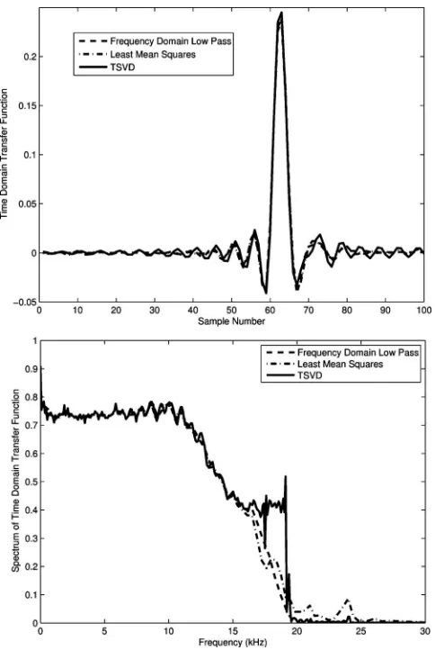
The forward going transfer functions obtained using these three techniques共frequency domain low pass deconvo-lution, LMS, and TSVD兲 are shown in the time and fre-quency domains in Fig. 3. An intermicrophone distance of L= 21.9 cm was used in a cylindrical tube of diameter 9.7 mm which extended for 149.1 cm after the last microphone. The signal to noise ratio became prohibitive above around 22 kHz. Theq共␻兲 vector for Eq.共3兲was chosen to equal 1 for frequency bins between 0 Hz and 16 kHz and then followed the half cosine profile over the range between 16 and 22 kHz, and then equal to zeros for the frequency bins between

0 0.002 0.004 0.006 0.008 0.01 0.012 0.014 0.016 −0.2

−0.1 0 0.1 0.2 0.3 0.4

S

ystem

Impulse

Response

Time (Seconds)

Microphone 1 Microphone 2

22 kHz and Nyquist at 48 kHz in order to generate the “Fre-quency Domain Low Pass” data with low noise. An advan-tage of the LMS technique is that it does not require prior knowledge of the bandwidth, but the number if samples in the derived filter may be entered. In this case 256 samples were used with a step size of ␮= 0.01. The TSVD results were obtained by fine tuning the condition number 共as de-scribed in Ref.15兲to cond= 45. This technique results in an extended bandwidth but the changeover from the passband to the stopband is sudden.

In the time domain the transfer functions are approxi-mately impulsive in shape with a delay due to time taken for sound to propagate between the microphones. Some energy appears to arrive before the main pulse in all cases due to ripple whose frequency is determined by the highest fre-quency in the bandwidth. The ripple is necessary to represent an impulse at a noninteger sample number and the width of the ripple in the time domain is inversely related to the ratio of the transition bandwidth and the sample rate. The fre-quency domain deconvolution approach has the least ripple in the time domain plot due to the smooth nature of the transition band in the frequency domain. This in turn means that the intermicrophone distance can be minimized without the first sample in the time domain filter becoming nonzero.

B. Causality and time domain windowing

Even a relatively short 共33 cm兲 length of tubing posi-tioned after the last microphone will separate the time do-main transfer function between microphones from the effect of secondary reflections in the resulting deconvolution. In order to prove that this is the case we need to consider how the two signals consist of an input pulse followed after a number of samples by secondary reflections. First let us label the signal recorded at microphone 1 when the source tube is terminated in an infinite pipe as s共n兲 共which is causal, i.e., zero for negative values ofn兲. This input signal will depend on the loudspeaker, microphone, and propagation character-istics as well as the excitation. In practice the signal at mi-crophone 1 will consist of s共n兲followed by multiple reflec-tions from the source tube ends:

p₁共n兲=s共n兲+s共n兲丢共rR共n兲+rR共n兲丢rL共n兲+rR共n兲

丢rL共n兲丢rR共n兲+¯兲, 共4兲

where 丢 denotes time domain convolution, rR共n兲 is the im-pulse response of the system to the right hand side of micro-phone 1, andrL共n兲 is the impulse response of the system to the left of microphone 1.

If the cylindrical pipe on the end of the source tube gives a total lengthl1 after the first microphone, then the multiple

reflections cannot start until M1= 2l1Fs/c samples later, wherecis the speed of sound andFsis the sample rate. This gives a practical signal in the form:

p₁共n兲=s共n兲+s共n−M₁兲丢r₁共n兲, 共5兲

wherer₁共n兲is a causal multiple reflection response obtained by expressing the bracket in Eq. 共4兲 with the time delay of M₁samples removed. Taking theztransform gives the signal in the form:

P1共z兲=S共z兲·共1 +z−M1R1共z兲兲, 共6兲

whereR1共z兲is thez transform of r1共n兲, etc. Similarly thez

transform of the signal at microphone 2 will be

P2共z兲=S共z兲·H12共z兲·共1 +z−M2R2共z兲兲, 共7兲

whereH12共z兲 is the z transform of the transfer function for

forward going waves between microphone 1 and microphone 2,R2共z兲is theztransform of the共causal兲multiple reflections

from the source tube ends as measured at microphone 2, and M2= 2l2Fs/c is the number of samples before the multiple reflections start. This is determined using l2, the distance

from the second microphone to the end of the cylindrical pipe. In generalM2⬎M1 because microphone 1 is closer to

the source, meaning that microphone 2 will receive reflec-tions from the opposite end of the source tube after a shorter time delay.

Dividing these two signals in thezdomain gives

P₂共z兲

P1共z兲

=H12共z兲·

1 +z−M2_R 2共z兲

1 +z−M1_R 1共z兲

. 共8兲

This can be rearranged to show the desired filterH12共z兲plus

the remaining energy due to multiple reflections:

FIG. 3. Transfer functions for frequency domain deconvolution, LMS, and TSVD shown in the time domain and frequency domains.

P2共z兲

P1共z兲

=H12共z兲+

H12共z兲共z−M2R2共z兲−z−M1R1共z兲兲

1 +z−M1_R 1共z兲

. 共9兲

Now as long as there is some loss of energy from the system then兩R1共z兲兩⬍1 for all frequencies and the formula

1

1 −a= 1 +a+a

2_+a3_{+¯ 共10兲}

can be used with the substitutiona= −z−M1_R

1共z兲to give

P2共z兲

P₁共z兲=H12共z兲+H12共z兲·共z

−M_2R

2共z兲−z−M1R1共z兲兲

⫻共1 −z−M_1R

1共z兲+z−2M1R21共z兲−¯兲. 共11兲

This formula shows how the secondary reflections only ef-fect the resulting deconvolution after M2 samples where

M2⬎M1. The tail of the response features a decaying

feed-back sequence with a delay time ofM1samples. It is

neces-sary that the number of samples in the deconvolution is great enough to resolve all of this decaying sequence 共otherwise the end of the sequence will show up as aliases at the start of the time domain兲. This can be achieved by zero padding in the time domain, although this was not necessary in the cur-rent experiments due to the large order chosen in using the sine sweep impulse response measurement technique. As long as the microphone frequency responses are similar, the desired filter关h₁₂共n兲兴 will be close to impulsive. There will always be some ripple in practical experiments which may be minimized by applying a low pass filter in the frequency domain, as described in Eq.共3兲. The resulting band limited impulse may then be isolated from the secondary reflections by windowing in the time domain with minimal error.

This theory holds for the frequency domain deconvolu-tion method. While it may be possible to extend this theory to use an adaptive filter approach, applying the LMS method to extended time domain signals gives unstable results due to secondary reflections being interpreted as errors in the algo-rithm. The LMS technique, however, can provide very good results provided that the signals can be truncated to remove secondary reflections. In the experiments that follow fre-quency domain deconvolution was used in calculating for-ward and backfor-ward going transfer functions due to the fact that this minimizes the length of calibration tube required共in this case a distance of 33 cm after the last microphone兲.

If the microphones have significantly different fre-quency responses, or one is poorly mounted in the wall of the source tube compared to the other, then the resulting deconvolution will not be close to being impulsive and a much longer length of tubing would be required after the last microphone. It should be noted this causality theory results in length requirements which are much less strict than pre-viously assumed in pulse reflectometry, where the source tube lengths are usually set to separate undeconvolved sys-tem impulse responses共which are much longer than decon-volved data兲.

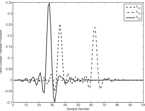
Figure4shows the results of performing the deconvolu-tion method in Eq.共3兲and time windowing to obtain all the possible time domain transfer functions for forward going waves in a system of M= 3 microphones. The

intermicro-phone distances wereL12= 12.5 cm andL23= 9.4 cm where

Labis the distance from microphonea to microphoneb and the cylindrical pipe extended for 33 cm after the last micro-phone.

The longer the intermicrophone distance, the wider the resulting time domain transfer function due to the attenuation at high frequencies in the source tube. In terms of digital signal processing, this can be viewed as a low pass finite impulse response filter, in that using it for convolution delays the signal and adds adjacent samples to smooth high fre-quency sounds out of the result.

V. BACKWARD GOING TIME DOMAIN TRANSFER FUNCTION

If the microphone gains were identical and the micro-phone signals were sampled simultaneously rather than in sequence, then the time domain transfer function for back-ward going waves from microphone 2 to microphone 1 would be identical. This is true, even if the loudspeaker is coupled differently at either end, as the transfer function de-scribes the transfer between microphones, rather than an ab-solute timing for travel from the speaker. Since the gains are generally not exactly the same the backward going response can be measured by repeating the measurement with the loudspeaker and calibration tube reversed.

Alternatively, we could express the forward going trans-fer function in terms of the theoretical acoustic transtrans-fer func-tion for travel between the microphones and the frequency dependent microphone gains. The frequency domain intermi-crophone transfer function from miintermi-crophone 1 to micro-phone 2 may be labeled ase−⌫d where⌫ is the propagation factor 共j multiplied by the complex wavenumber兲 and d is the distance between microphones, while the gain for micro-phone 1 may be labeledG1共␻兲, and the gain for microphone

2 labeledG2共␻兲. The frequency domain version of the

inter-microphone transfer function from inter-microphone 1 to micro-phone 2 becomes

H12共␻兲=e−⌫dG2共␻兲/G1共␻兲. 共12兲

Then we similarly express the backward going frequency domain transfer function as

0 10 20 30 40 50 60 70 80 90 100

−0.1 −0.05 0 0.05 0.1 0.15 0.2 0.25 0.3 0.35

Sample Number

Time

Domain

Trans

fer

Function

h

12

h₁₃ h₂₃

H21共␻兲=e−⌫dG1共␻兲/G2共␻兲. 共13兲

Multiplying the two equations to cancel the gain terms gives

H₂₁共␻兲=e−2⌫d/H₁₂共␻兲, 共14兲

whereH12共␻兲=F共h12共n兲兲 is known from the windowed

for-ward going calibration. This allows the calculation of the backward going time domain transfer function共following an inverse Fourier transform兲using a theoretical expression for the complex acoustic propagation constant without measur-ing it directly. Such a calculation should include losses due to interaction with the tube walls 共e.g., due to Keefe18兲. At high frequency the accuracy is further improved by including the effect of internal losses as shown in Ref. 3. The disad-vantage of using a theoretical expression is that the losses in the system cannot be calculated to perfect accuracy, as they are temperature and humidity dependent, and the audio hard-ware may be scanning the inputs sequentially, rather than sampling simultaneously. For this reason, two calibration measurements were made in the results which follow, to ob-tain maximum accuracy: one for the forward going case and one for the backward going case, with the loudspeaker and calibration tube interchanged between these measurements. This means that no assumption or prior knowledge is needed in relation to the intermicrophone distances, the location of the acoustic center of the microphones in relation to their geometric center, the synchronization between sound card inputs and the speed of sound, or any acoustic propagation coefficients, so long as they remain constant during the ex-periment.

As long as both the forward and backward going transfer functions are known then the acoustic intermicrophone trans-fer function and microphone gain ratio can be deduced from the measurement by rearrangement of Eqs. 共12兲 and 共13兲. The relative microphone gain 共which includes the effect of nonsimultaneous sampling in the sound card兲 can be found by dividing in the frequency domain to give

G2共␻兲

G₁共␻兲=

冑

H12共␻兲

H₂₁共␻兲, 共15兲

while the acoustic intermicrophone transfer function can be deduced by multiplying in the frequency domain to give

e−⌫d=

冑

It should be noted that an ambiguity has to be resolved in taking square roots in the frequency domain, which can be achieved by phase wrapping 共i.e., minimizing the phase angle rotation between adjacent frequency bins兲.

VI. TIME DOMAIN CONVOLUTION

If we initially assume that waves are traveling in only one direction, then we can use the time domain transfer func-tions to predict a signal at one microphone from the signal measured at another using convolution.

First, we measure the system impulse response at the first microphone,p₁共n兲, and at the second microphone,p₂共n兲, where the object under test is placed on the end of the source tube opposite the loudspeaker. Next, we define the vectors

for the forward going and backward going waves at the first microphone which we will label p₁+andp₁− and the forward and backward going waves at the second microphone which we will labelp₂+andp₂−.

Suppose that we have measured a signal at microphone 1 and know that it consists only of forward going waves. If we have our measured time domain transfer function for for-ward going travel from microphone 1 to 2共h12关n兴兲 which is

defined for discrete time sample numbers n= 1 , 2 , . . . ,Nf, then we can work out the expected forward going wave sig-nal at microphone 2:

p₂+关n兴=共h12丢p1+兲关n兴=

兺

m=1

N_f

共h12关m兴·p+1关n−m+ 1兴兲. 共17兲

Next let us suppose that we have measured a signal at mi-crophone 2 and also know that it consists only of backward going waves. If we have our measured time domain transfer function for forward going travel from microphone 2 to 1 共h21关n兴兲 which is defined for discrete time sample numbers

n= 1 , 2 . . .Nf then we can work out the expected backward going wave signal at microphone 1:

p₁−关n兴=共h21丢p2

−_兲关

n兴=

兺

m=1

N_f

共h21关m兴·p2 −_关

n−m+ 1兴兲. 共18兲

VII. WAVE SEPARATION USING TWO MICROPHONES

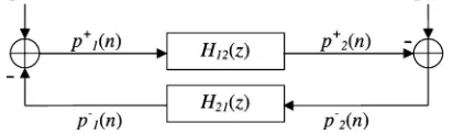
So far, it is not at all obvious how this type of analysis can be used to work out the forward going and backward going waves once they are overlapping. The key to this is causality. It is first assumed that all microphone signals start with silence, that they have been silent for at least Nf samples before sampling started共whereNfis the number of samples in the time domain transfer functions兲, and that ini-tially there are no acoustic waves traveling in the air con-tained in the source tube. The forward and backward going wave vectors for the microphone signals are then initialized to zero. It is also useful to insertNf− 1 zeros before the start of the impulse responses measured at the microphones,p₁共n兲 andp₂共n兲in order that time domain convolution共which nec-essarily involves looking backward in the time domain兲can be performed without running out of samples. Wave separa-tion is performed using a time domain loop using a signal processing procedure which is similar to digital waveguide modeling.19 This procedure is shown as a flow diagram in Fig. 5. It should be noted that Hab共z兲 denotes time domain convolution with the transfer functionhab.

FIG. 5. Flow diagram representation of the two microphone time domain wave separation algorithm.

For this algorithm to be computable, the first sample in h12must be zero, as otherwise a delay-free loop results. This

is equivalent to saying that no forward going wave energy gets to microphone 2 from microphone 1 within the space of one time sample. This would imply that the microphones must be at leastc/Fsapart whereFs is the sample rate共i.e., roughly 3.5 mm apart at 96 kHz兲. In practice, however, the bandwidth of the low pass filter used in the deconvolution implies a certain width of transfer function which, in turn, limits the minimum intermicrophone distance to around 9 cm for the current experiment. As long as this is the case, then the value ofp₁+共n兲is multiplied byh12共1兲= 0 in the

convolu-tion, so is not actually influencing the calculation and the use of p₁+共n兲before its definition is unimportant.

The technique relies on there being no forward or back-ward going wave present between the microphones at the start time for the analysis so that any nonzero signal received at the right hand microphone first may be assumed to be traveling backward and any signal received at the left hand microphone first may be assumed to be traveling forward.

It should be noted that applying the technique using two microphones involves poor handling of errors. Any errors in the measurement共such as an incorrect dc level, random noise or cross-talk between channels兲will show up as false predic-tions of forward or backward going waves. Due to the use of convolution these will not be constrained within one point in the time domain, but will lead to the error reappearing at a later time in the predictions of forward and backward going waves at the other microphone. If an error is sufficiently bad,

then equal and opposite oscillations共with a frequency deter-mined by the time of travel between microphones兲, may be seen in the predicted forward and backward going waves after the measured signals have died away to zero. The in-termicrophone travel time isL12/cand the expected

oscilla-tion has a period of twice this value giving the system a weakness at a frequency ofc/共2L12兲. This frequency is also a

problem for other two microphone techniques.

VIII. WAVE SEPARATION USING MORE THAN TWO MICROPHONES

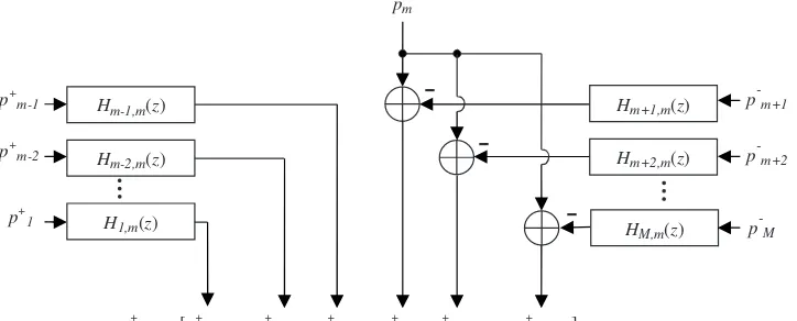
It is possible, and indeed desirable, to generalize the technique to use M microphones. This procedure is repre-sented by the flow diagrams in Figs. 6 and7. The forward and backward going waves at all microphones depend on the previous states of the incoming forward or backward going waves at all of the other microphones. At each time step in the wave separation algorithm then, the forward going and backward going waves at each of the M microphones are estimated by time domain convolution of each of the M− 1 incoming waves with the appropriate time domain transfer function. All predictions of backward going waves are then subtracted from the appropriate measured microphone sig-nals to convert them into predictions of the forward going wave.

The result is M− 1 predictions of the forward going wave at each microphone. These values are stored in a ma-trix,g+_{, which has dimensionM− 1 byM such that the} col-FIG. 6. Flow diagram representation of the M microphone time domain wave separation algorithm. The for-ward going wave at each microphone is found by taking the median of the corresponding column vector from the matrix g+_{. Time domain convolution} operations are used to calculateg+_as defined in Fig.7.

g+

*,m= [g+1,m,… g+m-2,m,g+m-1,m,g+m,m, g+m+1,m,… g+M-1,m]

-Hm+1,m(z)

HM,m(z)

pm

Hm+2,m(z)

-Hm-1,m(z)

Hm-2,m(z)

H1,m(z) p-M

p-m+2

p-m+1

p+

m-1

p+

m-2

p+

1

umn vectorg+_ⴱ,mwill store the M− 1 predictions of the for-ward going wave at the mth microphone. The simplest procedure for obtaining a single estimate of the forward go-ing waves at each microphone would be to take the average, but taking the median 共or 50 percentile兲is advantageous in that it ignores outlying values ifM⬎3. Once this procedure is done the backward going wave at each microphone at the current time step is obtained by taking the difference be-tween the measured signal and the forward going wave. The algorithm will then carry on to the next time step. In the absence of errors all the entries ing+_ⴱ,mshould be the same. Errors can thus be checked by taking the standard deviation of such a vector.

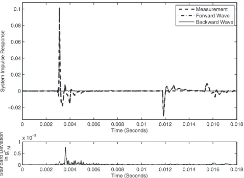
Figure8shows the results of applying the wave separa-tion algorithm with L12= 12.5 cm and L23= 9.4 cm for M

= 3 microphones. The measured microphone responses were low pass filtered with a cutoff of 16 kHz before being fed into the wave separation algorithm as this was the highest frequency in the passband for the transfer function measure-ments. For this measurement the cylindrical source tube was extended such that a cylinder of length 149.1 cm was present after the last microphone. This assured that the forward and backward going waves are clearly separated in time so that the effectiveness of the algorithm can be assessed. The mea-sured data consists of the microphone signal meamea-sured at the microphone furthest from the loudspeaker pM共n兲 with the forward gong wave being pM

+_共

n兲 and the backward going wave being pM

−_共

n兲. It may be observed that the input pulse passes the microphone at around 3 ms and the calculated forward going wave matches the measured microphone sig-nal at this point. The calculated backward going wave the matches the measured microphone signal at around 12 ms when the negative reflection from the end of the cylinder under test return to the microphone. After 15 ms the forward going reflections of this energy from the loudspeaker are observed. Also shown is the standard deviation in column vectorg+_ⴱ,Mas a function of time. The small values indicate that the predictions of the forward going waves at micro-phone 3 as derived using forward going convolution from microphone 1 and microphone 2 are in close agreement.

IX. APPLICATIONS

To summarize the experimental procedure, a swept sine system impulse response measurement is performed, with a loudspeaker on one end of the source tube and a calibration tube of matching internal diameter on the other end, and the forward going intermicrophone time domain transfer func-tions are deduced. Next the measurement is repeated, with the loudspeaker and calibration tube reversed, to deduce the backward going intermicrophone time domain transfer func-tions. Finally, the measurement is performed with an arbi-trary object and/or source at either end of the source tube and, as long as the experiment begins in silence, the forward going and backward going waves can be deduced using the wave separation algorithm.

In the analysis above we have discussed the signals p1

andp2, etc., as though the system impulse responses were the

actual waves recorded at the microphones although, in our current application, the actual recordings are often of sine sweep nature. This is possible because the result of doing a sine sweep measurement, and deconvolving to give the sys-tem impulse response, is equivalent to the excitation of the instrument by an impulse 共but with very a low noise floor兲. The wave separation technique described will in principle also work with undeconvolved sine sweep signals, or any other excitation 共as long as the time domain transfer func-tions have been measured successfully, preferably using swept sine input impulse response measurement兲. In prin-ciple, the current method could work with the apparatus used as a cylindrical section within a musical wind instrument bore under playing conditions, but it would be desirable to develop a way of adapting the calibration data to changing temperature to make the technique robust for this purpose as suggested by van Walstijnet al.17,20The greatest accuracy is expected to be obtained when applying wave separation to impulse response measurements, as any errors tend to accu-mulate with the number of samples analyzed and impulse response measurements have the useful data constrained over a minimum number of time samples.

A. Input impedance measurements

Perhaps the most obvious application for wave separa-tion is to place the loudspeaker at one end of the source tube and an object under test at the other end. In this case a high quality reflectance共i.e., frequency domain impulse response兲 measurement of the system to one side of the last micro-phone can be performed by deconvolving the forward and backward going waves in the source tube using frequency domain deconvolution:

R共␻兲= PM

−_共␻兲

PM

+_共␻兲. 共19兲

Herep_M+共␻兲andp_M−共␻兲are the discrete Fourier transforms of the forward and backward going pressure waves, respec-tively, at the last 共i.e., Mth兲 microphone. From the impulse response, the normalized input impedance can be calculated from the input impulse response as21

0 0.002 0.004 0.006 0.008 0.01 0.012 0.014 0.016 0.018 −0.02

0 0.02 0.04 0.06 0.08 0.1

Time (Seconds)

System

Impulse

Response

0 0.002 0.004 0.006 0.008 0.01 0.012 0.014 0.016 0.018 0

0.5 1x 10

−3

Time (Seconds)

S

tandard

Deviation

in

g

+ *,M

Measurement Forward Wave Backward Wave

FIG. 8. Wave separation for M= 3 microphones with L12= 12.5 cm and L23= 9.4 cm.

Z

¯_共␻兲= 1 +R共␻兲

1 −R共␻兲. 共20兲

The input impedance is defined as the ratio of the pressure amplitude and volume velocity amplitude for a sinusoidal input, so players can produce strong pressure resonances at frequencies close to peaks in input impedance. As it stands the apparatus is not designed for this purpose, as the input impedance is deduced at the plane of the microphone rather than at the end of the source tube. One way to work out the input impedance at the plane at the end of the source tube is to use an impedance projection. The disadvantage of this is that it is necessary to know the distance from the microphone to the end of the source tube and the propagation constant.

An alternative is to make an impulse response measure-ment on the system to one side of the last microphone with the source tube closed in a perfectly reflecting cap, and de-convolving this from the measurement of the object under test. As this cap measurement will consist of a single impulse there will be no singular frequencies, and this technique will work to remove the effect of the delay and losses in the source tube, as with conventional pulse reflectometry.

Figure 9 shows the input impedance of an open ended section of pipe of length 149.1 cm measured using the tech-nique, with M= 3 microphones and inter-microphone dis-tances ofL12= 12.5 cm andL23= 9.4 cm. Also shown is the

theoretical input impedance of a tube closed at one end and with an ideal open end at the other. The agreement is very good and only deviates below 100 Hz; this deviation may be due to the microphone spacing being small compared to the object length.

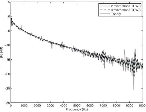
Since input impedance measurements have a high dy-namic range it is helpful to view the reflectance for the same system to assess accuracy. Figure10shows the magnitude of the reflectance for a tube of length 149.1 cm, closed at the end, and measured using M= 3 microphones 共with L₁₂ = 12.5 cm and L₂₃= 9.4 cm兲 and M= 2 microphones ob-tained by using the signals measured at microphones 1 and 3 共spaced 21.9 cm apart兲. These were calculated by using the time domain wave separation algorithm and deconvolving

the resulting forward and backward going waves using Eq.

共19兲with the resulting plots expressed in decibels. The effect of singularities can be seen in the two microphone data at integer multiples ofc/共2d兲⬇780 Hz. The three microphone calculation clearly reduces the effect of singularities signifi-cantly, with the reflectance showing a much improved agree-ment with theory up to 10 kHz. It is expected that using M = 4 microphones will provide an even greater improvement as there will then be three estimates of the incoming waves at each time step, meaning that the median procedure can ig-nore outlying values.

B. Comparison with frequency domain analysis

The wave separation results demonstrated thus far in this work have been computed using time domain processing. In terms of signal processing, the frequency domain and time domain versions of this wave separation process may be ex-pected to produce almost identical results for two micro-phone postprocessing. Description of the frequency domain version of the wave separation process in this section will demonstrate this equivalence in addition to illustrating how the intermicrophone transfer functions encode the losses and frequency dependent gain ratios. The analysis in De Sanctis and van Walstijn20for two microphones can be reformulated using the current calibration method to give a measured for-ward going wave at microphoneb of

Pb

+_共␻兲

=Hab·Pa共␻兲−e

−2⌫d ·Pb共␻兲

1 −e−2⌫d , 共21兲

where d=Labis the distance between the two microphones and Hab is the Fourier transform of the windowed forward going time domain transfer function共i.e., from microphonea to microphone b兲. If both the forward and backward going transfer functions have been measured then the propagation between microphones can be re-expressed entirely in terms of measured quantities by rearranging Eq.共14兲to give

0 200 400 600 800 1000 1200 1400 1600 1800 2000 −1.5

−1 −0.5 0 0.5 1 1.5

Frequency (Hz)

Ph

ase

A

ng

le

0 200 400 600 800 1000 1200 1400 1600 1800 2000 10−1

100 101

Frequency (Hz)

Absolute

Value

Normalised Input Impedance

TDWS Theory

TDWS Theory

FIG. 9. Input impedance of an open ended cylindrical tube of length 149.1 cm.

0 1000 2000 3000 4000 5000 6000 7000 8000 9000 10000 −30

−25 −20 −15 −10 −5 0 5

Frequency (Hz)

|R

|

(dB)

2 microphone TDWS 3 microphone TDWS Theory

e−2⌫d=Hab共␻兲·Hba共␻兲. 共22兲

It should be noted that the value of e−2⌫d cannot be deter-mined fromHab

2

unless the microphone signals are calibrated such that the forward and backward transfer functions are the same. Substituting into Eq. 共21兲 produces a measured for-ward going wave of

Pb

+_共␻兲

=Hab共␻兲·Pa共␻兲−Hab共␻兲Hba共␻兲·Pb共␻兲 1 −Hab共␻兲·Hba共␻兲

. 共23兲

The reflectance can then be derived as

R共␻兲= Pb

−_共␻兲

Pb

+_共␻兲=

Pb共␻兲−Pb

+_共␻兲

Pb

+_共␻兲

= Hab共␻兲·y共␻兲− 1

Hab共␻兲·Hba共␻兲−Hab共␻兲·y共␻兲

, 共24兲

and the normalized input impedance can be calculated using the above result as follows:

Z ¯

b共␻兲=

1 +R共␻兲 1 −R共␻兲

= Hab共␻兲·Hba共␻兲− 1

Hab共␻兲·Hba共␻兲+ 1 − 2Hab共␻兲·y共␻兲

, 共25兲

wherey共␻兲=Pa共␻兲/Pb共␻兲.

The reflectance derived using time domain processing wave separation and using an entirely frequency based analy-sis is shown in Fig.11. The time domain data was computed using M= 2 microphones and processing the forward and backward going waves using Eqs. 共19兲 and 共20兲. For the frequency domain the same experimental and calibration data was analyzed with Eq. 共24兲and the equivalence forM = 2 microphones of the time domain and frequency domain wave separation analysis is clear. An intermicrophone dis-tance ofd= 21.9 cm was used in each case and the effect of singularities at integer multiples of c/共2d兲⬇780 Hz can be clearly seen in the resulting figure.

C. Test object bore reconstruction

Input impulse response measurements can also be used to calculate the bore profile using the lossy layer peeling algorithm by Amir et al.22 In order to do this the input im-pulse response must be expressed in the time domain. This can be done using the equation

r共n兲=F−1

冉

PM

+_共␻兲q共␻兲

冊

where q共␻兲 is a smoothly varying frequency domain low pass filter vector to compensate for the bandwidth of the apparatus as described in Eq.共3兲. As with previous deconvo-lution procedures, the LMS filter can be used instead without previous knowledge of the bandwidth.

As shown in Sec. IX A, the accuracy of the current tech-nique is best above 100 Hz. Low frequency components have a significant effect on the bore reconstruction algorithm5and for this reason the low frequency components in the input impulse response were interpolated progressively toward⫺1 below this frequency before using the bore recon-struction algorithm. Alternative approaches for analyzing the data include using an optimization procedure to obtain con-vergence between the reconstructed bore’s theoretical and measured impedance.23

Figure12shows the bore reconstruction calculated with the lossy layer peeling algorithm for a Smith Watkins trum-pet lead pipe 共model 10兲 using three microphone time do-main wave separation, again with intermicrophone distances of L12= 12.5 cm and L23= 9.5 cm. The dimensions of the

mandrel used during manufacture are superimposed. Also shown are the external measurements and internal exit diam-eter measured using calipers.

Previous bore reconstruction studies using pulse reflec-tometry have shown Gibb’s oscillations close to steps in the bore due to the finite bandwidth of the experiment while small leaks lead to expansions in the bore whose gradient depends on the size of the leak.4Some Gibb’s oscillations of

0 200 400 600 800 1000 1200 1400 1600 1800 2000 −14

−12 −10 −8 −6 −4 −2 0 2

Frequency (Hz)

|R

|

(dB)

TM2C

2 microphone TDWS Theory

FIG. 11. Magnitude of the reflectance of an open ended cylindrical tube of length 149.1 cm for two microphone wave separation in the frequency do-main共TM2C兲and time domain共TDWS兲.

0 50 100 150 200 250

8 8.5 9 9.5 10 10.5 11 11.5 12 12.5 13

Axial Position (mm)

Diameter

(mm

)

Three Microphones Mandrel External Diameter Inside Exit Diameter

FIG. 12. Bore reconstruction of No. 10 leadpipe by Smith Watkins calcu-lated from a three microphone measurement. Also shown are the diameter of the mandrel used in manufacture, the external profile of the crook, and internal exit diameter measured with calipers.

amplitude⫾0.25 mm are present in the bore reconstruction at the exit of the tube in Fig. 12with the average value of these oscillations matching the internal exit diameter to within 0.1 mm. The agreement between the bore reconstruc-tion and the mandrel used in manufacture is clear and shows that there are no leaks in the object under test. The external diameter measurements also show a convincing agreement with the slope of the data, given the fact that the wall thick-ness contributes around 2⫻0.45 mm2_{to the external}

diam-eter measurement at the exit.

X. CONCLUSIONS

The time domain wave separation technique developed here forMmicrophones has proved to be successful in using measured transfer functions to track forward and backward going waves in a cylindrical pipe using time domain convo-lution. This technique has been applied to produce bore re-construction and input impedance measurements. Two cali-brations are required to measure the forward and backward going intermicrophone transfer functions. High bandwidth measurements using a relatively compact source tube can then follow. As with the existing multiple microphone tech-niques by van Walstijnet al.3and Dickenset al.,2the current method does not require assumptions or prior knowledge of the intermicrophone distances, or the location of the acoustic center of the microphones in relation to their geometric cen-ter. While the two microphone version of the algorithm suf-fers from singularities, these may be overcome by using three or more microphones, as with existing frequency do-main techniques. The current calibration technique has the advantage of using only two load free calibration measure-ments for an arbitrary number of microphones by reversing the source tube for backward going calibration. This calibra-tion procedure is illustrated to work in both time and fre-quency domain formulations.

Since the technique employs time domain windowing of pulselike signals, it represents the first multimicrophone re-flectometry method. In contrast to frequency domain ap-proaches, that for M microphones typically combine the re-sults of M− 1 separate measurements using different microphone distances, the proposed method combines the information of M microphone signals within a single time domain structure. The effects of singularities are effectively suppressed by calculating the pressure wave value at each time step for each of the microphones as the median of M − 1 forward-wave predictions that are obtained via time do-main convolution. This current approach has been found to be effective, but it has not yet been investigated whether it provides the optimal solution to the overdetermined system. Future work in this field should include an investigation of the behavior of the current algorithm for M⬎3 in compari-son to least squares approaches, particularly that of Jang and Ih.8

ACKNOWLEDGMENTS

We wish to acknowledge Dr. Noam Amir at the Univer-sity of Tel Aviv for helpful discussions on the use of medians and Dr. Barbara Forbes for providing source code for TSVD calculations.

1_{J. P. Dalmont, “Acoustic impedance measurement, Part I: A review,” J.}

Sound Vib.243, 427–439共2001兲.

2_{P. Dickens, J. Smith, and J. Wolfe, “Improved precision in measurements}

of acoustic impedance spectra using resonance-free calibration loads and controlled error distribution,” J. Acoust. Soc. Am.121, 1471–1481共2007兲. 3_{M. van Walstijn, M. Campbell, J. Kemp, and D. Sharp, “Wideband}

mea-surement of the acoustic impedance of tubular objects,” Acta. Acust. Acust.91, 590–604共2005兲.

4_{D. Sharp and M. Campbell, “Leak detection in pipes using acoustic pulse}

reflectometry,” Acta. Acust. Acust.83, 560–566共1997兲.

5_{A. Li and D. Sharp, “The problem of offset in measurements made using}

acoustic pulse reflectometry,” Acta. Acust. Acust.91, 789–796共2005兲. 6_{J. Buick, J. Kemp, D. Sharp, M. van Walstijn, M. Campbell, and R. Smith,}

“Distinguishing between similar tubular objects using pulse reflectometry, a study of trumpet and cornet leadpipes,” Meas. Sci. Technol.13, 750–757

共2002兲.

7_{N. Amir, O. Barzelay, A. Yefet, and T. Pechter, “Condenser tube}

exami-nation using acoustic pulse reflectometry,” ASME J. Eng. Gas Turbines Power132, 014501共2010兲.

8_{S. Jang and J. Ih, “On the multiple microphone method for measuring}

in-duct acoustic properties in the presence of mean flow,” J. Acoust. Soc.

Am.103, 1520–1526共1998兲.

9_{G. Piñero and L. Vergara, “Separation of forward and backward acoustic}

waves in car exhaust by array processing,” in ICASSP-95, 1995 Interna-tional Conference on Acoustics, Speech, and Signal Processing 共1995兲,

Vol.3, pp. 1920–1923.

10_{A. Seybert, “Two-sensor methods for the measurement of sound intensity}

and acoustic properties in ducts,” J. Acoust. Soc. Am. 83, 2233–2239

共1988兲.

11_{J. Guerard and X. Boutillon, “Real-time wave separation in a cylindrical}

pipe with applications to reflectometry and echo-cancellation,”J. Acoust. Soc. Am.103, 3010共1998兲.

12_{P. Nauclér and T. Söderström, “Separation of waves governed by the}

one-dimensional wave equation—A stochastic systems approach,” Mech. Syst. Signal Process.23, 823–844共2009兲.

13_{S. Müller and P. Massarani, “Transfer-function measurement with}

sweeps,” J. Audio Eng. Soc.49, 443–471共2001兲.

14_{J. Kemp, J. Chick, D. M. Campbell, and D. Hendrie, “Acoustic pulse}

reflectometry for the measurement of horn crooks,” in Acoustics ’08, Paris

共2008兲.

15_{B. Forbes, D. Sharp, J. Kemp, and A. Li, “Singular system methods in}

acoustic pulse reflectometry,” Acta. Acust. Acust.89, 743–753共2003兲. 16_{B. Farhang-Boroujeny,Adaptive Filters: Theory and Applications共Wiley,}

Chichester, NY, 1998兲.

17_{M. van Walstijn and G. de Sanctis, “Towards physics-based re-synthesis of}

woodwind tones,” in 19th International Congress on Acoustics, Madrid, Spain共2007兲.

18_{D. Keefe, “Acoustical wave propagation in cylindrical ducts: Transmission}

line parameter approximations for isothermal and nonisothermal boundary conditions,” J. Acoust. Soc. Am.75, 58–62共1984兲.

19_{J. O. Smith, “Physical modelling using digital waveguides,” Comput.}

Mu-sic J.16, 74–91共1992兲.

20_{G. de Sanctis and M. van Walstijn, “A frequency domain adaptive}

algo-rithm for wave separation,” in 12th International Conference on Digital Audio Effects共DAFx-09兲, Como, Italy共2009兲.

21_{D. Sharp, “Acoustic pulse reflectometry for the measurement of musical}

wind instruments,” Ph.D. thesis, University of Edinburgh, UK共1996兲. 22_{N. Amir, G. Rosenhouse, and U. Shimony, “A discrete model for tubular}

acoustic systems with varying cross section—The direct and inverse prob-lems. Parts 1 and 2: Theory and experiment,” Acustica 81, 450–474

共1995兲.

23_{W. Kausel, “Bore reconstruction of tubular ducts from its acoustic input}