C
2012. The American Astronomical Society. All rights reserved. Printed in the U.S.A.
THE EFFECTS OF LINE-OF-SIGHT INTEGRATION ON MULTISTRAND CORONAL LOOP OSCILLATIONS
I. De Moortel and D. J. Pascoe
School of Mathematics and Statistics, University of St. Andrews, North Haugh, St. Andrews, Fife KY16 9SS, UK;[email protected]
Received 2011 October 13; accepted 2011 December 23; published 2012 January 23
ABSTRACT
Observations have shown that transverse oscillations are present in a multitude of coronal structures. It is generally assumed that these oscillations are driven by (sub)surface footpoint motions. Using fully three-dimensional MHD simulations, we show that these footpoint perturbations generate propagating kink (Alfv´enic) modes which couple very efficiently into (azimuthal) Alfv´en waves. Using an ensemble of randomly distributed loops, driven by footpoint motions with random periods and directions, we compare the absolute energy in the numerical domain with the energy that is “visible” when integrating along the line of sight (LOS). We show that the kinetic energy derived from the LOS Doppler velocities is only a small fraction of the actual energy provided by the footpoint motions. Additionally, the superposition of loop structures along the LOS makes it nearly impossible to identify which structure the observed oscillations are actually associated with and could impact the identification of the mode of oscillation.
Key words: magnetohydrodynamics (MHD) – Sun: atmosphere – Sun: corona – Sun: oscillations – waves
Online-only material:color figures
1. INTRODUCTION
Historically, the dissipation of (MHD) waves and oscillations in the corona has been invoked as one way to provide (some of) the energy needed to account for the unexpectedly high coronal temperatures (several orders of magnitude higher than the solar surface; see reviews by, e.g., Walsh & Ireland2003; Klimchuk
2006; or Taroyan & Erd´elyi2009). Although direct observations of waves and oscillations in the solar corona were absent for a long time, recent observations have revealed that a variety of small amplitude oscillations is present in almost all coronal structures. Alongside their possible role in coronal heating, MHD waves can be used as a seismological tool (Uchida
1970; Roberts et al.1984) to provide estimates of local plasma
parameters that are difficult to obtain by direct measurements (see reviews by, e.g., De Moortel2005; Nakariakov & Verwichte
2005; Erd´elyi 2006; Banerjee et al. 2007; or De Moortel &
Nakariakov 2012). The recent confirmation of the ubiquitous
presence of waves and oscillations in the solar atmosphere by, for example, Tomczyk et al. (2007) and McIntosh et al. (2011), is likely to substantially widen the possible application of coronal seismology and has reopened the debate on the role of wave heating in the solar atmosphere. The identification of the correct mode and the estimate of the energy budget will play a crucial role in both of these applications. Of particular interest in the coronal heating debate are the observations in the past few years of transverse oscillations propagating along the magnetic field in a variety of structures such as prominences (Okamoto et al.
2007), X-ray jets (Cirtain et al.2007), spicules (De Pontieu et al.
2007; He et al. 2009a, 2009b), and coronal loops (Tomczyk
et al.2007; Tomczyk & McIntosh2009; McIntosh et al.2011).
Also, Jess et al. (2009) reported on the possible detection of
torsional Alfv´en waves in the lower solar atmosphere, with an energy budget that could be sufficient to account for the coronal heating requirements.
As the solar corona is optically thin, line-of-sight (LOS) integration means that in any given pixel of, for example, an EUV image, several coronal structures are likely to be present and this has to be taken into consideration when interpreting the
observations. For example, the effect this LOS integration has on the appearance of coronal structures in EUV observations
is discussed by DeForest (2007). Tomczyk et al. (2007) have
shown that small amplitude transverse oscillations are likely to be present in a large number of (off-limb) coronal loops
and Tomczyk & McIntosh (2009) briefly discuss the effect
of the LOS superposition and resolution on the estimated
energy budget. Similarly, McIntosh et al. (2011) point out
that the estimated energy budgets they report are likely to be lower limits, due to LOS superposition. Cooper et al.
(2003) considered the effects of LOS integration on a single
loop and demonstrated how this could potentially complicate the identification of observed oscillations. For example, the largely incompressible kink mode could still be associated with perturbations in the emission, depending on the angle
between the loop and the LOS. Terradas et al. (2008) look
at resonant absorption in a similar multistrand model but these authors focus on the actual resonant absorption process and do not consider the consequences of the LOS integration. In this paper, we investigate the effects of LOS superposition in a three-dimensional (3D) numerical model of a multistrand structure. We make a qualitative, order of magnitude comparison between the “observed” energy budget (from Doppler shift oscillations), which will be greatly reduced due to the LOS superposition, with the energy budget actually present in the loop oscillations. We also address the issue of mode identification, especially in light of the recent observations of ubiquitous Doppler shift perturbations propagating in coronal loops.
The paper is organized as follows. The setup is described in Section2, the results are analyzed in Section3, and a discussion
and conclusions are presented in Section4.
2. MODEL SETUP
We consider a straight magnetic field in the (vertical)
z-direction and choose the background plasma β = 0.01 to
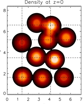
Figure 1.Contours of a horizontal cross section of the density (i.e., as a function ofxandy). The horizontal dashed and vertical dot-dashed lines represent the locations of density enhancements which appear to be loop structures when integrating overxory, respectively (see also Figure2).
(A color version of this figure is available in the online journal.)
magnitude grounds, i.e., sufficiently high to actually allow for LOS superposition but small enough for the numerical resolu-tion to be sufficiently high to resolve the mode coupling process. A high numerical resolution is needed to ensure that the phase-mixed Alfv´en waves (generated by the mode coupling process) do not reach scales below the grid resolution. Each individual loop is set up as in Pascoe et al. (2010); a vertical cylindrical tube, with a core region of constant density, surrounded by an inhomogeneous layer (referred to as the tube boundary or shell
region). The density isρ0 in the core region andρein the
ex-ternal region (r > a). We choose density contrastsρ0/ρein the
range 2.5–4, and an inhomogeneous layer thicknessl/a=0.75.
Figure1 shows a contour plot of the cross section of the
den-sity at the base of our simulation (z = 0). The 10 loops with
different density contrasts are clearly identifiable. Note that we are considering a coronal volume in our numerical simulations as the aim of this paper is to illustrate how estimates of the
energy budget derived from observedcoronalDoppler shift
os-cillations (Tomczyk et al.2007; Tomczyk & McIntosh2009)
are affected by the optically thin LOS superposition. Each loop
has a temperature profile similar to that for density:T0 in the
core region,Tein the external region, and varying linearly in
the inhomogeneous region. We choose a temperature contrast ratio ofT0/Te=1.1 for all loops. In order to produce an
equi-librium for our hot and dense loops, we vary the magnitude of the magnetic field strength so as to satisfy the condition of to-tal pressure balance. Consequently, the magnetic field strength is up to 2% smaller inside the loops than outside. Inside the
loops, the plasmaβ rises up to 0.043. All variables have been
non-dimensionalized using typical values for the magnetic field strengthB0, the densityn, and a typical lengthscaleL0.
2.1. Driver
The driving condition is applied to the lowerzboundary to
simulate excitation by random footpoint motions. Our driver generates transverse velocity perturbations propagating along field lines. By placing our driver at the bottom of the coronal domain, we are trying to mimic observed Doppler shift oscil-lations. Although we are implicitly assuming these footpoint motions are related to solar surface motions, we do not consider
the propagation of these oscillations through the atmosphere. Theoretically, our driver corresponds to moving the loop foot-point back and forth about its initial position, which is a very general perturbation that could be generated by a number of pro-cesses. The time dependence of our driver is based on a single
period displacement of the loop axis as in Pascoe et al. (2010)
and is applied from t = 0 to t = P0. This lower boundary
driving generates a non-monochromatic propagating wavetrain along each loop, with the dominant period of oscillation in a
Fourier spectrum beingP ≈ 23P0. Each loop has its own
par-ticular value of driving timeP0, randomly chosen in the range
13.5–16.5. A single pulse has been chosen rather than (possibly more realistic) continuous or quasi-periodic driving to keep the perturbations and their associated energy budgets tractable. Al-though continuous driving would be a more accurate reflection of solar surface motions, the effect of the optically thin LOS integration on the estimated energy budget and the mode iden-tification will be essentially the same. Indeed, the single pulse used in this study to illustrate the LOS effects could be seen as a single wavelength (or driving period) of a (harmonic) wavetrain or quasi-periodic wavepacket and the mode coupling process has more or less the same effect on a single wave pulse as it does on a harmonic wavetrain. The spatial dependence of the driver is based on a two-dimensional dipole (see Pascoe et al.
2010,2011) and each loop has a direction of oscillation
ran-domly chosen in thex–y-plane. The maximum amplitude of the
transverse velocities at the lower boundary is chosen to be small (u0/CAe =0.01) to approximate a linear regime.
The simulations are performed using the MHD codeLare3D
(Arber et al. 2001) with 400×400 ×300 grid points for
a numerical domain of 70 ×84×500 Mm. The boundary
conditions are periodic in thex- andy-directions, and are placed sufficiently far away to not affect the results. Initially the lower
zboundary is driven, but after our driving phase (t P0) the
driver is turned off and thezboundaries also become periodic.
This avoids the need for a large domain in the field-aligned direction by allowing the wavetrain to propagate out of the top of our domain and re-enter at the lower boundary. We remind the reader that, throughout this manuscript, non-dimensional values of all parameters are used. Dimensional quantities can be obtained by assuming a normalizing value of the magnetic fieldB0, a typical lengthscaleL0, and number density ρ0 (see
Arber et al.2001). For example, using a value ofB0 =10 G,
L0 =10 Mm, andρ0 =1015m−3gives a timescale oft0=14.5 s. Hence with this normalization the periods of 13.5–16.5 would correspond to 200–240 s.
3. EFFECTS OF LINE-OF-SIGHT INTEGRATION
3.1. Density (Intensity) Structures
Ten different flux tubes are present in the numerical domain and these 10 individual structures are clearly identifiable in
the horizontal cross section shown in Figure 1. However,
superposition along the LOS effectively means summing some of these structures together. To simulate optically thin intensity,
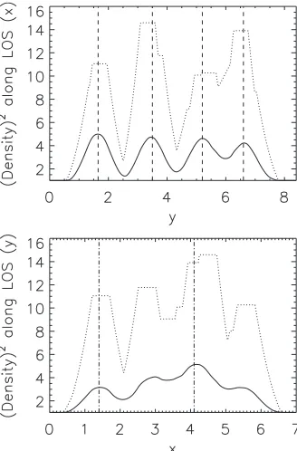
the top panel of Figure2shows a cross section of the density
squared, integrated along the x-direction (and subsequently
divided by the appropriate number of gridpoints to avoid artificially high values of density). As indicated by the vertical dashed lines, there are four clearly distinct maxima and hence
when thex-direction coincides with the LOS (i.e., an observer
is placed further along the x-axis), only 4 loops would be
Figure 2.Cross section of the average density squared (i.e., divided by the number of gridpoints) integrated along thex-direction (top panel) andy-direction (bottom panel). The vertical dashed (dot-dashed) lines identify the maxima and correspond to the horizontal dashed (vertical dot-dashed) lines in Figure1. The dotted lines correspond to the maximum value of the density squared in the 3D numerical domain at eachy(x).
the 3D domain. Similar integration along they-direction reduces
the number of “visible” loops to two as indicated by the
dot-dashed lines in the bottom panel of Figure2. The positions of
the maxima in the LOS integrated intensities (density squared)
are also presented in Figure 1 as horizontal dashed lines
(corresponding to the x-LOS integration) and vertical
dot-dashed lines (y-LOS) to illustrate how the summations have
reduced the number of visible structures to four and two, respectively. Generally, the locations of the peaks in the averaged densities do not correspond exactly to the locations of the center of the loop structures present in the 3D domain. In no case does an LOS integrated “loop” actually correspond to a single loop
in the 3D domain. Also shown in Figure2by the dotted lines is
the maximum value of the density squared in the 3D numerical
domain at eachy(x). Comparing the dotted lines, which reflect
the actual intensity contrast (ρ0/ρe)2present in the domain, with
the solid lines, we notice that the LOS summation does not only confuse the location of the actual structures but substantially reduces the intensity contrasts. This is especially noticeable for
they-LOS, where the averaged LOS intensity appears almost
uniform. Hence, a region which appears nearly uniform, or with very low intensity contrast, could actually be a bundle of closely spaced loops with substantial density contrasts, implying that seismologically inferred density contrasts (from observed damping lengths) might not correspond well with the density (intensity) contrast visible in the LOS integrated observations.
3.2. LOS Doppler Velocities
As described in Section 2, each of the 10 structures is
now subjected to an oscillatory displacement at the base of our numerical domain. For a single loop, the resulting mode
coupling is described comprehensively by Pascoe et al. (2010,
2011); such perturbations travel along the loop and efficiently
couple to an azimuthal Alfv´en wave in the tube boundaries. This mode coupling process has been investigated in great detail recently (Pascoe et al.2010,2011; Terradas et al.2010; Verth et al.2010; Soler et al.2011a,2011b). What is important for our current investigation is that the damping length of the central, transverse displacement is (mainly) governed by the period of the footpoint driver, the density contrastρ0/ρe,
and the relative thickness of the tube boundary (Hollweg &
Yang1988; Goossens et al.1992; Ruderman & Roberts2002;
Pascoe et al. 2010; Terradas et al. 2010). The width of the
shell region is the same for all 10 loops but the driving periods and density contrasts are different for each of the loop structures. Hence, they will each have different damping lengths, implying that at any given height, a mixture of transverse
displacements and/or azimuthal Alfv´en waves, at different
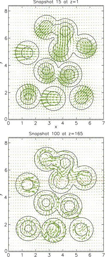
phases of oscillation, will be present: at low height, the velocity perturbations will be dominated by the transverse (kink) modes whereas at large heights, only the azimuthal Alfv´en waves will remain. At intermediate heights, both modes will be present and hence an integration along a given LOS will capture velocity perturbations that are a mixture of the transverse displacements and azimuthal Alfv´en modes, as both are linear combinations of vx andvy. To illustrate this, Figure3 shows the horizontal
velocity vectors in two different horizontal planes, at z = 1
(top) andz=165 (bottom) att =15 andt=100, respectively.
It is clear that the lower height (top panel) is dominated by the randomly directed, transverse displacements induced by the bottom boundary driver, whereas the higher plane (bottom panel) is dominated by the azimuthal perturbations in the loop boundaries. In other words, the energy has moved from the cores of the loops to the outer shell regions due to mode coupling of the driven kink modes to the (azimuthal) Alfv´en modes.
The LOS summation will make it difficult to uniquely identify individual structures (irrespective of the additional question of whether current observations actually resolve such structures) and hence it is already clear that it will be non-trivial to actually associate observed Doppler velocities with a given structure in the LOS. Additionally, as illustrated below, loop structures and their associated oscillations could line up in such a way
as to make the (azimuthalm = 1) Alfv´en waves in the tube
boundariesappearas larger bulk motions in the LOS integrated
density structures.
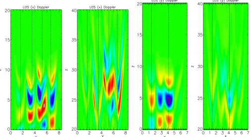
In Figure4, the LOS velocities that would be observed either
along the x- or y-axis are shown. These LOS velocities have
been calculated by averaging the density-squared weighted
velocity components along the LOS, i.e., ρ2vx,y/ρ2 for
the x, y LOS and where · · · represents the average along
the appropriate LOS. Zacharias et al. (2011) have shown (see
their Figure 4) that this intensity-weighted velocity accurately reflects Doppler shifts of optically thin emission lines. The first
two panels of Figure 4 correspond to the x-axis being the
LOS and the colored contours represent vx, integrated over
x. Observationally, these perturbations would correspond to
periodic Doppler velocities traveling along magnetic structures (loops). As oppositely directed perturbations in the LOS will cancel each other out, the resulting Doppler velocities will be much smaller than the actual values in the numerical domain.
For thex-LOS, the resulting Doppler velocities appear to line
Figure 3.Velocity vectors in the horizontal plane att = 15 (z = 1) and t=100 (z=165). The line contours correspond to the density and outline the loop structures. Note that the vectors in both panels havenotbeen scaled to a common maximum.
(A color version of this figure is available in the online journal.)
oscillations), but would appear to be occurring in the wing of
a wide structure (see the bottom panel of Figure2). At early
times, both the x and y integrated velocities would mainly
correspond to the (bulk) transverse loop motions induced by the footpoint driver. At later times (i.e., higher heights), the remaining velocity perturbations are much weaker and mostly situated in the tube boundaries, as illustrated in the bottom
panel of Figure3. However, when integrated along the LOS,
the azimuthal motions in the shell regions of neighboring loops could appear as bulk motions of the central part of an integrated
loop. This has occurred in thex-LOS where, at y = 5.2, an
apparent bulk motion is still visible at later times. However,
closer inspection of the planar velocities at, e.g., z = 27.5
reveals that what appears to be a bulk Doppler velocity along
the LOS loop centered on y = 5.2 is mainly composed of
the azimuthal Alfv´en waves in the boundary of the flux tube
centered on [x =1.4, y =4.9] (see horizontal dashed line in
the bottom panel of Figure3).
3.3. Energy Budget
Finally, we focus on the effect of the LOS integration on
the (apparent) energy budget. Figure5shows the evolution of
the horizontal kinetic energy, i.e., only the horizontal velocity
componentsvxandvy have been taken into account. The solid
line corresponds to this horizontal kinetic energy integrated over the full 3D numerical domain at each timestep. The dashed and dot-dashed lines represent the LOS kinetic energies, obtained by using the LOS intensity-weighted velocity components (the summedρ2vx,y/ρ2), multiplied by the appropriate average
density (see Figure2). It is clear that using the observed Doppler velocity along either LOS combined with the averaged density will underestimate the energy that is actually present in the
3D domain, by as much as an order of magnitude. In the y
-direction, the kinetic energy is never more than 40% of the total
kinetic energy present in the 3D domain, whereas the x-LOS
only gives about 10%. In addition, the transverse driving of the loop footpoints will also result in magnetic perturbations and hence magnetic energy. The magnetic energy present in the numerical domain is of the same order as the kinetic energy, implying that the total energy contained in the transverse perturbations is double of the kinetic energy alone (see the dotted line in Figure5). Hence, the (kinetic) energies estimated from the LOS Doppler velocities would only capture 5%–20% of the energy actually present in the 3D domain. It is clear that energy estimates based on observed Doppler velocities could underestimate the actual energy present in footpoint-driven (transverse) loop oscillations by at least one, possibly two if more loops are considered, orders of magnitude. It is important to keep in mind that the LOS integrated energy cannot easily be associated with the different wave modes (either the transverse, propagating kink waves or the azimuthal Alfv´en waves generated by the mode coupling). Indeed as shown by
Pascoe et al. (2010) (see their Figure 9), there is a gradual
energy transfer for each loop from the transverse mode in the core to the Alfv´en waves in the shell region. Hence, apart from the very lowest heights in our numerical domain, where almost all the energy will be in the boundary-driven kink mode, the LOS integrated energy will contain a mixture of the kink mode and Alfv´en wave contributions until all the energy from the kink mode in the core has been transferred to the azimuthal Alfv´en waves in the shell regions.
4. DISCUSSION AND CONCLUSIONS
Even though their interpretation has been under debate, it has become clear that propagating, transverse oscillations are present in most observed coronal structures. Having success-fully been modeled as coupled kink and (azimuthal) Alfv´en waves (e.g., Pascoe et al.2010; or Terradas et al.2010), these “Alfv´enic” waves appear to contain sufficient energy to account for the quiet-Sun and solar wind requirements (McIntosh et al.
2011). As they appear to be present all the time, in large
Figure 4.LOS velocity perturbations integrated overx(left panels) andy(right panels) att=30 (panels 1 and 3) andt=100 (panels 2 and 4). The colored contours correspond the integratedvxandvyvalues. The vertical (dot-)dashed lines correspond to the maxima in the averaged LOS densities as indicated in Figure2. Note that
the maxima in the panels at later times have been scaled tohalfthe value of the maxima at earlier times to make the perturbations visible. (A color version of this figure is available in the online journal.)
Figure 5.Normalized energy as a function of numerical timesteps. The solid line correspond to the kinetic energy in the 3D numerical domain whereas the dotted line corresponds to the total energy, i.e., kinetic plus magnetic energy, in the 3D numerical domain. The dashed and dot-dashed lines correspond to the kinetic energy resulting from thex- andy-LOS integrated velocities, respectively.
Using a simple model of 10 randomly distributed loops, driven by randomly directed footpoint displacements, our sim-ulations are intended to demonstrate how the LOS integration of optically thin emission lines could affect the identification of observed oscillations as well as the energy budgets. As sev-eral loop structures in the LOS are likely to be superimposed, associating observed Doppler velocities (i.e., the components of the velocity perturbations which are directed (anti-)parallel to the LOS) with specific structures is non-trivial. Additionally, the dependence of the damping length of the driven kink mode (through mode coupling) on the density contrast, driving period, and loop (transverse) structure means that the perturbations will
have different damping lengths in different loops and hence integrated velocities are likely to contain a mixture of (bulk) transverse velocities from the cores of the loops and (azimuthal) Alfv´en perturbations from the loop boundaries. The interpreta-tion of these oscillainterpreta-tions as “Alfv´enic” appears attractive not only from a theoretical point of view (to reflect the generic cou-pled character of the mode) but also from an observational point of view (as the observed Doppler shift oscillations are likely to contain a mixture of kink and azimuthal Alfv´en waves at any given height). In this study, estimating the energy based only on the integrated LOS intensity-weighted velocity components (representing Doppler shifts of optically thin emission lines) un-derestimates the energy actually present in the 3D domain, by as much as an order of magnitude (and possibly two orders of magnitude if the magnetic energy associated with the perturba-tions is included in the full 3D energy budget). In any case, there will be more energy available to couple to the Alfv´en waves in the loop boundaries and ultimately, through the process of phase mixing, to heat the coronal loops than LOS estimates based on observed coronal Doppler shift oscillations might suggest.
[image:5.612.61.277.398.550.2]et al.2007; Tomczyk & McIntosh2009). The damping lengths of the propagating, transverse perturbations (or in other words the rate at which energy will be transferred from the transverse oscillations in the core to the Alfv´en waves in the shell regions of the loop) strongly depend on the period and the density contrast. Higher frequencies and stronger density contrasts will lead to shorter damping lengths. Hence, considering a wider range of these parameters will result in a wider range of damping lengths present in the domain. This would imply that, at any given height, an even greater mixture of the kink and azimuthal Alfv´en waves would be present in the LOS. The structure of the driver will also play a crucial role. In our setup, we considered a driver with a spatial scale equal to the cross section of the individual loop strands. As the direction of the transverse driving for each loop was chosen randomly, this leads to significant cancellation of the velocity perturbations along the LOS. If on the other hand all loops are driven in the same way, i.e., the spatial scale of the driver is considerably larger than the cross section of the loop strands, then all the loops will oscillate in phase and there will be no cancellation of velocity perturbations along the LOS. A final important factor is of course the number of loops present along the LOS. This will depend both on the location of the loop oscillations and on the spatial resolution of the observations. For off-limb loop oscillations and instruments with lower spatial resolution (COMP) the effects will be biggest as there is likely to be a large number of loops present along the LOS and within a single pixel. For on-disk observations of, e.g., a quiet-Sun region, the effects are likely to be much smaller. This is consistent with the findings of Tomczyk & McIntosh
(2009) and McIntosh et al. (2011): the energy flux contained
in off-limb COMP (lower spatial resolution) observations of quasi-periodic Doppler shift oscillations was found to be several orders of magnitude smaller than similar quiet-Sun observations
of transverse perturbations made bySDO/AIA.
In summary, the effects of the LOS integration depend on a large number of factors. It is likely that, in reality, far more than 10 loop strands will be present in the LOS, especially in active regions and/or off-limb observations and additional effects such as curvature would also have to be taken into account. Indeed, more complicated (curved) structures will further enhance the effects we have described. Our results also imply that properties
derived through coronal seismology are likely to reflect averaged properties of an ensemble of coronal loops.
I.D.M. acknowledges support of a Royal Society Univer-sity Research Fellowship. D.J.P. acknowledges financial sup-port from STFC. Computational time on the Linux clusters in St. Andrews (STFC and SRIF funded) is gratefully acknowl-edged. The authors thank Drs. H. Peter and S. McIntosh for valuable discussions.
REFERENCES
Arber, T. D., Longbottom, A. W., Gerrard, C. L., & Milne, A. M. 2001,J. Comput. Phys.,171, 151
Banerjee, D., Erd´elyi, R., Oliver, R., & O’Shea, E. 2007,Sol. Phys.,246, 3 Cirtain, J. W., Golub, L., Lundquist, L., et al. 2007,Science,318, 1580 Cooper, F. C., Nakariakov, V. M., & Tsiklauri, D. 2003,A&A,397, 765 DeForest, C. E. 2007,ApJ,661, 532
De Moortel, I. 2005,Phil. Trans. R. Soc. A,363, 2743
De Moortel, I., & Nakariakov, V. M. 2012, Phil. Trans. R. Soc. A, in press De Pontieu, B., McIntosh, S. W., Carlsson, M., et al. 2007,Science, 318,
1574
Erd´elyi, R. 2006,Phil. Trans. R. Soc. A,364, 289
Goossens, M., Hollweg, J. V., & Sakurai, T. 1992,Sol. Phys.,138, 233 He, J.-S., Marsch, E., Tu, C.-Y., & Tian, H. 2009a,ApJ,705, L217 He, J.-S., Tu, C.-Y., Marsch, E., et al. 2009b,A&A,497, 525 Hollweg, J. V., & Yang, G. 1988,J. Geophys. Res.,93, 5423
Jess, D. B., Mathioudakis, M., Erd´elyi, R., et al. 2009,Science,323, 1582 Klimchuk, J. A. 2006,Sol. Phys.,234, 41
McIntosh, S. W., De Pontieu, B., Carlsson, M., et al. 2011,Nature,475, 477 Nakariakov, V. M., & Verwichte, E. 2005, Living Rev. Solar Phys.,2, 3 Okamoto, T. J., Tsuneta, S., Berger, T. E., et al. 2007,Science,318, 1577 Pascoe, D. J., Wright, A. N., & De Moortel, I. 2010,ApJ,711, 990 Pascoe, D. J., Wright, A. N., & De Moortel, I. 2011,ApJ,731, 73 Roberts, B., Edwin, P. M., & Benz, A. O. 1984,ApJ,279, 857 Ruderman, M. S., & Roberts, B. 2002,ApJ,577, 475 Soler, R., Terradas, J., & Goossens, M. 2011a,ApJ,734, 80 Soler, R., Terradas, J., Verth, G., & Goossens, M. 2011b,ApJ,736, 10 Taroyan, Y., & Erd´elyi, R. 2009,Space Sci. Rev.,149, 229
Terradas, J., Arregui, I., Oliver, R., et al. 2008,ApJ,679, 1611 Terradas, J., Goossens, M., & Verth, G. 2010,A&A,524, A23 Tomczyk, S., & McIntosh, S. W. 2009,ApJ,697, 1384
Tomczyk, S., McIntosh, S. W., Keil, S. L., et al. 2007,Science,317, 1192 Uchida, Y. 1970, PASJ,22, 341
Verth, G., Terradas, J., & Goossens, M. 2010,ApJ,718, L102 Walsh, R. W., & Ireland, J. 2003,A&AR,12, 1