Instabilities in the spin up of a rotating, stratified fluid

(1)

R. J. Munro, M. R. Foster, and P. A. Davies

Citation: Physics of Fluids 22, 054108 (2010); doi: 10.1063/1.3422554 View online: http://dx.doi.org/10.1063/1.3422554

View Table of Contents: http://scitation.aip.org/content/aip/journal/pof2/22/5?ver=pdfcov Published by the AIP Publishing

Articles you may be interested in

Instabilities and waves on a columnar vortex in a strongly stratified and rotating fluid Phys. Fluids 25, 086601 (2013); 10.1063/1.4816512

Elliptical instability of a rapidly rotating, strongly stratified fluid Phys. Fluids 21, 074104 (2009); 10.1063/1.3177354

Nonaxisymmetric effects of stratified spin-up in an axisymmetric annular channel Phys. Fluids 17, 086601 (2005); 10.1063/1.2002999

Long-time evolution of linearly stratified spin-up flows in axisymmetric geometries Phys. Fluids 17, 016601 (2005); 10.1063/1.1834570

Short-wavelength instabilities of waves in rotating stratified fluids Phys. Fluids 10, 3168 (1998); 10.1063/1.869843

(2)

Instabilities in the spin-up of a rotating, stratified fluid

R. J. Munro,1,a兲 M. R. Foster,2and P. A. Davies3 1

Environmental Fluid Mechanics Research Group, Process and Environmental Research Division, Faculty of Engineering, University of Nottingham, Nottingham NG7 2RD, United Kingdom 2

Department of Aerospace Engineering, The Ohio State University, Columbus, Ohio 43210, USA 3

Department of Civil Engineering, University of Dundee, Dundee DD1 4HN, United Kingdom

共Received 23 June 2009; accepted 13 April 2010; published online 26 May 2010兲

Theoretical analyses and laboratory experiments have been performed on the stability of a flow generated by the differential cyclonic corotation of a flat, rigid disk in a uniformly rotating, linearly stratified fluid contained within a cylindrical tank. The undisturbed fluid is stably stratified with salt 共Schmidt number␴⬇670兲and the共vertical兲axes of rotation of the disk and the fluid container are coincident. The theoretical analysis shows that when the interior flow satisfies gradient wind balance 共or, alternatively, thermal wind balance兲, it is destabilized by the action of viscosity. In the experiments, the manifestation of the viscous overturning instability is seen to be the formation of steplike internal microstructures in the density field, observed as regularly spaced, curved ring-shaped sheets with associated localized sharp, vertical density gradients. A stability analysis of the flow shows that the instability criterion is dependent on local values of the vertical and radial gradients of zonal velocity and the background density field. These quantities are measured in the experiments using a combination of horizontal-plane particle image velocimetry and an array of traversing microconductivity probes. The stability criterion based on this linear analysis predicts that the interior of the fluid is unstable. Using the␴Ⰷ1 condition, simple asymptotic expressions for the maximum growth rate and associated wave number have been derived from the cubic dispersion relation. The theoretically predicted length scales and e-folding times associated with the fastest growing modes are found to give excellent agreement with the corresponding values obtained from the laboratory experimental data. ©2010 American Institute of Physics.关doi:10.1063/1.3422554兴

I. INTRODUCTION

The term spin-up is commonly used to describe the pro-cess by which a bounded fluid in a state of solid-body rota-tion responds to a change in external forcing induced by an increase in rotation rate of the flow boundaries共or, in some cases, a specific region of the flow boundary兲. Given the significance of spin-up to the dynamics controlling many at-mospheric and oceanographic flows共in which the effects as-sociated with the Earth’s rotation are important and often dominant兲, a considerable amount of research has been dedi-cated to analyzing the spin-up problem for both homoge-neous and stratified fluids, as well as for a range of flow geometries and configurations. Much of this previous work to date is described in the review articles by Benton and Clarke1 and, more recently, by Duck and Foster.2

This article further investigates the “double-diffusive” instability associated with the spin-up of a stably stratified fluid; a mechanism first identified by McInytre.3,4 The ex-periment configuration we use to study this instability 共 de-scribed in detail in Sec. III兲 consists of a cylindrical tank containing a stably stratified water solution which is initially in a state of solid rotation, with the axis of rotation coinci-dent with the central symmetry axis of the cylinder. At time t= 0, relative motion within the fluid is induced by the rota-tion of a smooth, flat, rigid, horizontal disk posirota-tioned at the

tank base and set to rotate uniformly, coaxially, and cycloni-cally共viz., in the same direction as the background rotation兲. Various processes have been studied using this, similar or related configurations. Typical examples include theoretical aspects of stratified spin-up,5,6mixing and frontogenesis,7–11 and internal waves.12

McInytre3discovered the theoretical basis of the double-diffusive instability when investigating the properties of a steady axisymmetric zonal shear flow in a thermally strati-fied annulus. Local linear stability theory was used to show that when the background flow is in geostrophic balance, and provided that␴⫽1 共where for thermal and saline stratifica-tions ␴ denotes the Prandtl and Schmidt numbers, respec-tively兲, the flow can be destabilized by the disparity in dif-fusion coefficients of momentum and density of the fluid, giving rise to relatively small-scale axisymmetric overturn-ing motions.

At about the same time, and using an experiment setup similar to one the described here, Baker13 provided experi-mental evidence of McIntyre’s instability for a salt-stratified fluid. Baker13 used the shadowgraph technique to visualize the instability, which manifests itself as a regular density step 共or staircase兲 microstructure superimposed on the back-ground density field.关A shadowgraph image showing a typi-cal density microstructure observed in our experiments is given in Fig. 5共a兲.兴 Baker13 used measurements obtained directly from the shadowgraph images to compare with McIntyre’s instability criteria for the ␴Ⰷ1 limit. A similar

a兲_{Electronic mail: rick.munro@nottingham.ac.uk. Telephone:} _⫹₄₄ _共₀_兲₁₁₅

9513893.

(3)

analysis was performed by Calman,14although improved ex-perimental data were obtained using a single conductivity probe 共to sample the fluid density field兲 and dye lines 共to estimate the zonal velocity field兲.共There is also speculative evidence for the occurrence of this double-diffusive instabil-ity in the study by Hedstrom and Armi.15兲

This paper describes experiments used to investigate, in detail, the development of McIntyre’s diffusive instability. Following the approach of Baker,13our experiments consider the spin-up of a linearly stratified, salt water solution by the differential rotation of a horizontal disk. The focus was on obtaining detailed measurements of how the fluid density and velocity fields共and associated gradients兲develop as the instability forms, with an emphasis on obtaining significantly improved spatial and temporal resolution in comparison with the relatively primitive measurements obtained by Baker13 and Calman.14 This was achieved using an array of high-frequency response conductivity probes to measure the fluid density field and particle image velocimetry共PIV兲 to mea-sure the zonal-plane velocity field共at different heights within the fluid兲. McIntyre’s linear stability theory is also reformu-lated in the context of this experimental setup. We then use the dispersion relation in the␴Ⰷ1 limit to derive asymptotic results for the most unstable normal mode. Maximum growth rates and corresponding wave numbers are then compared with observations.

II. LINEAR STABILITY THEORY

In anticipation of the cylindrical geometry used in our experiments, let 共r,␪,z兲 denote the cylindrical coordinate system which rotates with constant angular velocity ⍀zˆ about the verticalz-axis aligned antiparallel to the gravita-tional acceleration vector −gzˆ. Relative to this rotating refer-ence frame, we consider a steady, axisymmetric zonal shear flowu共r,z兲=¯v共r,z兲␪ˆ of continuously salt-stratified water so-lution which is Boussinesq and in hydrostatic and gradient wind balance.关In this context, the term Boussinesq indicates that density variations are assumed negligible except in the buoyancy terms, and that the coefficients of viscosity 共␯兲, salinity diffusion共␬兲, and salinity contraction共␤兲 are taken to be constant共with frictional heating assumed negligible兲.兴 Moreover, we write the共dimensional兲 density and pressure fields as

␳共r,z兲=␳s共z兲+␳0␤s¯共r,z兲, 共1a兲

p共r,z兲=ps共z兲+¯p共r,z兲, 共1b兲

where␳_s共z兲andp_s共z兲denote the hydrostatic components,␳₀ is a constant reference density, and¯s共r,z兲 is the dimension-less salinity. The gradient wind balance 共or zonal vorticity equation兲, therefore, is given by

2共⍀+¯v/r兲¯vz= −g␤¯sr, 共2兲 where the subscript partial-derivative notation is standard. This basic flow-state will be assumed to remain stably strati-fied 共¯sz⬍0兲 and centrifugally stable 共¯vr⬎0兲 throughout. Note that the cylindrical nature of the flow means that Eq. 共2兲includes the nonlinear共centrifugal兲term 2¯vz¯v/r, which is

required to maintain the balanced state when the isobars are curved. However, it is worth noting that when curvature ef-fects are negligible, Eq. 共2兲 reduces to the thermal wind equation 2⍀¯vz= −g␤¯sr, which corresponds to the geostrophic balance. Indeed, it is this thermal wind balance that was used in the analysis of both McIntyre3and Calman.14However, it should be noted that the analysis which follows here is little affected by whether the background state is taken to be a gradient wind or a thermal wind balance.

McIntyre3showed that the basic balanced state described by Eqs.共1兲and共2兲, when otherwise stable according to the classical inviscid criterion, can become unstable provided that ␴=␯/␬⫽1. In the present case, that of a salt-stratified water solution with Schmidt number␴⬇670, the destabiliz-ing agent is viscosity. That is, the relative absence of salinity diffusion 共in comparison with momentum diffusion兲 means that a fluid element that is perturbed from its initial balanced state will be brought into momentum equilibrium by the ac-tion of viscous torques significantly faster than the density of the element is able to adjust to the ambient buoyancy of its new surroundings. Therefore, any local density difference induced by this double-diffusive mechanism can give rise to meridional overturning motions共i.e., zonal vorticity兲, the ba-sic source of this instability. Moreover, the instability mecha-nism is of a localized nature, not requiring for its function the presence of a flow boundary, or a free surface. Hence, adopting the approach taken by McIntyre,3we treat the basic flow as being unbounded and consider the local behavior of small-amplitude, axisymmetric perturbations about the back-ground balanced state described by Eqs.共1兲and共2兲.

The basic steady state is localized about an interior point 共r0,z0兲by introducing dimensionless meridional coordinates

共x,y兲and time␶defined, respectively, by

x=共r−r0兲/␦1, y=共z−z0兲/␦1, ␶=t/␶1, 共3兲

where the dimensional time and length scales␶₁ and␦₁ are chosen such that

␶1=共g␤¯sr0兲−1/2, ␦1=共␯/2⍀兲1/2␥−1/4, 共4兲

with the dimensionless parameter␥ defined as

␥=g␤s¯_r0/4⍀2_. _共₅_兲

In the above, the notation¯s0₌_¯_s_共_r

0,z0兲 has been used, and

will henceforth be adopted throughout, together with

v

¯0₌_¯_v_共_r

0,z0兲.关Note that using the balanced state given in Eq.

共2兲, we can also write␥= −共⍀r0+¯v0兲v¯z

0_/

2r0⍀2, and that␥is

the analogue of the dimensionless parameter defined in Eq. 共2.4d兲of McIntyre3共p. 24兲.兴

The background flow variables are then expanded about the interior point 共r0,z0兲 as ¯v=¯v0+⑀r0共x¯vr

0

+y¯v_z0兲共 like-wise for¯,s ¯vr,¯sr,¯vz, and¯sz兲, where ⑀=␦1/r0 and ⑀Ⰶ1 is

assumed. Therefore, neglecting termsO共⑀兲关and noting that 1/r= 1/r0共1 +⑀x兲= 1/r0+O共⑀兲兴, the linearized equations for

perturbations in momentum and density, about 共r0,z0兲, can

be written in dimensionless form as

冉

⳵

⳵␶−ⵜ2

冊

ⵜ2␺−vy−sx= 0, 共6a兲

(4)

冉

⳵

⳵␶−ⵜ2

冊

v−共⌰1␺y−␺x兲= 0, 共6b兲

冉

⳵

⳵␶−␴−1ⵜ2

冊

s−共⌰2␺x−␺y兲= 0, 共6c兲

where 共␺y,v, −␺x兲 and s denote 共dimensionless兲 perturba-tions in velocity and salinity, respectively,共each of which are assumed to be axisymmetric functions of x, y, and ␶兲, and ⵜ2_⬅_⳵2_/⳵_x2₊_⳵2_/_⳵_y2 _{is the standard Laplacian. Using}

conti-nuity, the stream function␺共x,y,␶兲 has been introduced to eliminate the dependence on the pressure perturbation by combining the radial and vertical momentum equations共 us-ing cross-differentiation兲 into the single Eq. 共6a兲 for the zonal component of vorticity,ⵜ2_␺_{. The dimensionless}

coef-ficient parameters in Eqs.共6兲are defined as

␴=␯/␬, 共7a兲

⌰1=共v¯r0+¯v0/r0+ 2⍀兲/¯vz0, 共7b兲

⌰2=共¯sz

0

−N₀2/␤g兲/s¯_r0, 共7c兲 which depend only on the system constants 共␯,␬,⍀兲, the buoyancy frequency N₀=关−共g/␳₀兲d␳s/dz兴1/2_{, and the local}

characteristics of the zonal flow and salinity fields. Finally, note that the final form of Eqs.共6兲are obtained by choosing the relative scales for the perturbation amplitudes such that

2共¯v0_/r

0+⍀兲vⴱ=␺ⴱ/共␶1␦1兲=g␤s, 共8兲

where the star superscript denotes the dimensional form the perturbation variables.

The linearized Eqs.共6兲support simple normal mode so-lutions of the form

共␺,v,s兲= exp关ik共xcos␾+ysin␾兲+␻␶兴, 共9兲 where the growth rate␻ 共which can be complex兲 is depen-dent on the wavenumber k and the wave-vector direction ␾ 共both of which are real兲. The basic state 共␴,⌰1,⌰2兲 is

therefore unstable if there exist values of 共k,␾兲 such that R共␻兲⬎0. Substituting Eq.共9兲 into Eqs. 共6兲 and setting the determinant of the resulting coefficient matrix to zero gives a cubic dispersion relation of the form

共␻+k2兲2共␻+k2/␴兲+共I+G兲␻+共I/␴+G兲k2= 0, 共10兲 where

I= 1₂sin 2␾−⌰1sin2␾, 共11a兲

G=1₂sin 2␾−⌰2cos2␾, 共11b兲

which depend only on the background flow characteristics and␾.

The form of the dispersion relation 共10兲 is the same as that derived by McIntyre,3 and we now take advantage of McIntyre’s analysis of Eq.共10兲. First, we see that the neces-sary criterion for classically subcritical flow to be I+G⬎0 for all values of␾; since by puttingk= 0 in Eq.共10兲with this condition we then obtain the roots␻= 0 ,⫾i共I+G兲1/2. More-over, McIntyre shows that for this classically subcritical flow

共i.e., withI+G⬎0 assumed兲, the necessary criterion for the diffusive instability described above can be obtained by con-sidering the real root of Eq.共10兲

␻= −k2共I/␴+G兲/共I+G兲+O共k6兲, 共12兲 where we have takenkⰆ1 for this approximation.

Specifically, there is monotonic instability if and only if there exist values of␾ such thatR共␻兲⬎0. Using Eq. 共12兲, this condition at leading order reduces toI/␴+G⬍0, which gives

⌰1⌰2⬍

␴ 4

冉

1 +

1 ␴

冊

2

. 共13兲

Furthermore, oscillatory instability occurs if and only if there exist ␾ such that R共␻兲⬎−k2_共_{2 + 1}_/␴_{兲共}_{for details, see}

McIntyre3兲. Again, using Eq.共12兲, this condition at leading order becomesI/␴+G⬎共2 + 1/␴兲共I+G兲, which gives

⌰1⌰2⬍

9 8

再

关1 +共1/3␴兲兴2

1 +共1/␴兲

冎

. 共14兲 We return to these theoretical results in Sec. IV, with analysis of the limiting case for large Schmidt number␴.

III. EXPERIMENTS

A. Experiment arrangement

Figure1shows a side view of the experiment apparatus. A cylindrical acrylic tank 共diameter 36 cm; height 30 cm兲 was fitted centrally inside an outer rectangular container 共thereby eliminating optical distortion caused by the curved sidewalls兲and mounted on a rotating turntable with the axis of the cylinder aligned through the vertical rotation axis of the table 共as shown兲. With the table initially stationary, the two tanks were filled to a depthH= 25 cm with a linearly salt-stratified water solution using the standard double-bucket system.16,17 Once filled and the fluid quiescent, the system was gradually brought to a state of solid-body rota-tion, with the desired angular frequency ⍀. To prevent ex-cessive mixing, the prescribed final solid rotation rate of the system共⍀兲 was attained using small incremental increases from rest over a time interval of about 7 hours.

Following the approach of Baker,13 the flow conditions required to observe the instability were established using a smooth disk of radius R= 17.5 cm 共and negligible thick-ness兲, set to rotate horizontally at the base of the cylindrical tank about a drive shaft mounted through the central axis of cylinder 共see Fig.1兲. The drive shaft was connected共via a water-tight seal兲 to an external motor positioned below the two tanks, allowing the disk to be rotated independently of the table with a predetermined共constant兲angular frequency ⍀d. The disk rotation 共in the same sense as the background

rotation of the system兲 was initiated at time t= 0, with the fluid in a state of solid rotation. Our cylindrical coordinates 共r,␪,z兲 are aligned so that the horizontal disk surface corre-sponds toz= 0, with the vertical z-axis directed through the central axis of the cylinder. In all cases, the time taken for the disk to reach a steady rotation rate was significantly less than one table rotation period共2␲/⍀兲.

(5)

Measurements of vertical profiles of fluid density were obtained using an array of three conductivity probes18 fitted on a vertical, motor-driven traverse mechanism above the cylinder, at radii r/R= 0 , 0.5, 0.9 共see Fig. 1兲. A personal computer共PC兲mounted on the turntable controlled the mo-tion of the traverse, together with acquisimo-tion and storage of the conductivity and probe-position data. When idle, the probes were located above the fluid with only the sampling tip submerged below the fluid surface. A single traverse mea-sured the vertical structure of fluid density over the range 0.04ⱕz/Hⱕ0.90 共during the downward stroke only兲, at these three radial locations. The traverse time and sampling frequency of the probes were 1.5 s and 200 Hz, respectively, giving density measurements approximately every 0.08 cm. The correspondence between conductivity and density was established empirically before each experiment, using a simple calibration procedure. During the initial period fol-lowing the onset of disk rotation, density measurements were taken at intervals of between 30 s and 2 min. The sampling frequency was progressively reduced throughout the experi-ment, as the flow conditions became quasisteady, to intervals of between 20 and 30 min during the later stages of the experiment.

The primary source of uncertainty in the density mea-surements was associated with inherent signal noise and the empirical conversion between conductivity to density. In all cases, the resulting variability in the density measurements obtained with the probes was negligible 共and always less than 10−3 g/cm3兲. Uncertainties in the probe response in-duced by thermal variations in the fluid共over the period of

each experiment兲, and the variability associated with the me-chanical measurements of probe position, were both found to be negligible in comparison to the above.共It is worth noting that the water used to fill the tanks was first allowed to reach the ambient temperature of the laboratory over a period of 24 hours; typical variations in the fluid temperature over the period of each experiment were always less than 1 ° C.兲

Measurements of the zonal velocity field were obtained, in four horizontal layers above the disk, using PIV. Small, neutrally buoyant tracer particles used to seed the fluid were illuminated by four horizontal light sheets positioned at fixed heights z/H= 0.12, 0.32, 0.52, and 0.72 共see Fig. 1兲. A cyclic timing device activated each light sheet individually 共for a set period of 30 s兲, while the remaining lights were switched off. This sequence was repeated indefinitely. The particle trajectories were recorded during each 30 s in-terval using a digital video camera共sampling at 24 Hz with 1380⫻512 pixel resolution兲 fastened to the turntable and positioned to view vertically down into the tank interior through a thin perspex lid used to eliminate free-surface dis-tortion 共see Fig. 1兲. The PC mounted on the turntable was used for image acquisition and storage, with the velocity fields calculated at the end of the experiment using PIV tech-niques developed by Dalziel.19 At each of the four fixed heights, the processed velocity data, denoted by u₁共x,y,t兲i

+u2共x,y,t兲j, were first calculated in terms of the Cartesian

coordinates systemx=rcos␪,y=rsin␪, and then converted to corresponding polar coordinates, denoted U共r,␪,t兲rˆ +V共r,␪,t兲␪ˆ, using the standard transformation

0 0 0 0 0 0 0 0 0 0 0 0 0 0 0 0 0 0 0 0 0 0 0 0 0 0 0 0 0 0 0 0 0 0 0 0 0 0 0 0 0 0 0 0 0 0 0 0 0 0 0 0 0 0 0 0 0 0 0 0 0 0 0 0 0 0 0 0 0 0 0 0 0 0 0 0 0 0 0 0 0 0 0 0 0 0 0 0 0 0 0 0 0 0 0 0 0 0 0 0 0 0 0 0 0 0 0 0 0 0 0 0 0 0 0 0 0 0 0 0 0 0 0 0 0 0 0 0 0 0 0 0 0 0 0 0 0 0 0 0 0 0 0 0 0 0 0 0 0 0 0 0 0 0 0 0 0 0 0 0 0 0 0 0 0 0 0 0 0 0 0 0 0 0 0 0 0 0 0 0 0 0 0 0 0 0 0 0 0 0 0 0 0 0 0 0 0 0 0 0 0 0 0 0 0 0 0 0 0 0 0 0 0 0 0 0 0 0 0 0 0 0 0 0 0 0 0 0 0 0 0 0 0 0 0 0 0 0 0 0 0 0 0 0 0 0 0 0 0 0 0 0 0 0 0 0 0 0 0 0 0 0 0 0 0 0 0 0 0 0 0 0 0 0 0 0 0 0 0 0 0 0 0 0 0 0 0 0 0 0 0 0 0 0 0 0 0 0 0 0 0 0 0 0 0 0 0 0 0 0 0 0 0 0 0

1 1 1 1 1 1 1 1 1 1 1 1 1 1 1 1 1 1 1 1 1 1 1 1 1 1 1 1 1 1 1 1 1 1 1 1 1 1 1 1 1 1 1 1 1 1 1 1 1 1 1 1 1 1 1 1 1 1 1 1 1 1 1 1 1 1 1 1 1 1 1 1 1 1 1 1 1 1 1 1 1 1 1 1 1 1 1 1 1 1 1 1 1 1 1 1 1 1 1 1 1 1 1 1 1 1 1 1 1 1 1 1 1 1 1 1 1 1 1 1 1 1 1 1 1 1 1 1 1 1 1 1 1 1 1 1 1 1 1 1 1 1 1 1 1 1 1 1 1 1 1 1 1 1 1 1 1 1 1 1 1 1 1 1 1 1 1 1 1 1 1 1 1 1 1 1 1 1 1 1 1 1 1 1 1 1 1 1 1 1 1 1 1 1 1 1 1 1 1 1 1 1 1 1 1 1 1 1 1 1 1 1 1 1 1 1 1 1 1 1 1 1 1 1 1 1 1 1 1 1 1 1 1 1 1 1 1 1 1 1 1 1 1 1 1 1 1 1 1 1 1 1 1 1 1 1 1 1 1 1 1 1 1 1 1 1 1 1 1 1 1 1 1 1 1 1 1 1 1 1 1 1 1 1 1 1 1 1 1 1 1 1 1 1 1 1 1 1 1 1 1 1 1 1 1 1 1 1 1 1 1 1 1 1 1

0 0 0 0 0 0 0 0 0 0 0 0 0 0 0 0 0 0 0 0 0 0 0 0 0 0 0 0 0 0 0 0 0 0 0 0 0 0 0 0 0 0 0 0 0 0 0 0 0 0 0 0 0 0 0 0 0 0 0 0 0 0 0 0 0 0 0 0 0 0 0 0 0 0 0 0 0 0 0 0 0 0 0 0 0 0 0 0 0 0 0 0 0 0 0 0 0 0 0 0 0 0 0 0 0 0 0 0 0 0 0 0 0 0 0 0 0 0 0 0 0 0 0 0 0 0 0 0 0 0 0 0 0 0 0 0 0 0 0 0 0 0 0 0 0 0 0 0 0 0 0 0 0 0 0 0 0 0 0 0 0 0 0 0 0 0 0 0 0 0 0 0 0 0 0 0 0 0 0 0 0 0 0 0 0 0 0 0 0 0 0 0 0 0 0 0 0 0

1 1 1 1 1 1 1 1 1 1 1 1 1 1 1 1 1 1 1 1 1 1 1 1 1 1 1 1 1 1 1 1 1 1 1 1 1 1 1 1 1 1 1 1 1 1 1 1 1 1 1 1 1 1 1 1 1 1 1 1 1 1 1 1 1 1 1 1 1 1 1 1 1 1 1 1 1 1 1 1 1 1 1 1 1 1 1 1 1 1 1 1 1 1 1 1 1 1 1 1 1 1 1 1 1 1 1 1 1 1 1 1 1 1 1 1 1 1 1 1 1 1 1 1 1 1 1 1 1 1 1 1 1 1 1 1 1 1 1 1 1 1 1 1 1 1 1 1 1 1 1 1 1 1 1 1 1 1 1 1 1 1 1 1 1 1 1 1 1 1 1 1 1 1 1 1 1 1 1 1 1 1 1 1 1 1 1 1 1 1 1 1 1 1 1 1 1 1

0

1

0 0 0 0 0 0 0 0 0 0 0 0 0 0 0 0 0 0 0 0 0 0 0 0 0 0 0 0 0 0 0 0 0 0 0 0 0 0 0 0 0 0 0 0 0 0 0 0 0 0 0 0 0 0 0 0 0 0 0 0 0 0 0 0 0 0 0 0 0 0 0 0 0 0 0 0 0 0 0 0 0 0 0 0 0 0 0 0 0 0 0 0 0 0 0 0 0 0 0 0 0 0 0 0 0 0 0 0 0 0 0 0 0 0 0 0 0 0 0 0 0 0 0 0 0 0 0 0 0 0 0 0 0 0 0 0 0 0 0 0 0 0 0 0 0 0 0 0 0 0 0 0 0 0 0 0 0 0 0 0 0 0 0 0 0 0 0 0 0 0 0 0 0 0 0 0 0 0 0 0 0 0 0 0 0 0 0 0 0 0 0 0 0 0 0 0 0 0 0 0 0 0 0 0 0 0 0 0 0 0 0 0 0 0 0 0 0 0 0 0 0 0 0 0 0 0 0 0 0 0 0 0 0 0 0 0 0 0 0 0 0 0 0 0 0 0 0 0 0 0 0 0 0 0 0 0 0 0 0 0 0 0 0 0 0 0 0 0 0 0 0 0 0 0 0 0 0 0 0 0 0 0 0 0 0 0 0 0 0 0 0 0 0 0 0 0 0 0 0 0 0 0 0 0 0 0 0 0 0 0 0 0 0 0 0 0 0 0 0 0 0 0 0 0 0 0 0 0 0 0 0 0 0 0 0 0

1 1 1 1 1 1 1 1 1 1 1 1 1 1 1 1 1 1 1 1 1 1 1 1 1 1 1 1 1 1 1 1 1 1 1 1 1 1 1 1 1 1 1 1 1 1 1 1 1 1 1 1 1 1 1 1 1 1 1 1 1 1 1 1 1 1 1 1 1 1 1 1 1 1 1 1 1 1 1 1 1 1 1 1 1 1 1 1 1 1 1 1 1 1 1 1 1 1 1 1 1 1 1 1 1 1 1 1 1 1 1 1 1 1 1 1 1 1 1 1 1 1 1 1 1 1 1 1 1 1 1 1 1 1 1 1 1 1 1 1 1 1 1 1 1 1 1 1 1 1 1 1 1 1 1 1 1 1 1 1 1 1 1 1 1 1 1 1 1 1 1 1 1 1 1 1 1 1 1 1 1 1 1 1 1 1 1 1 1 1 1 1 1 1 1 1 1 1 1 1 1 1 1 1 1 1 1 1 1 1 1 1 1 1 1 1 1 1 1 1 1 1 1 1 1 1 1 1 1 1 1 1 1 1 1 1 1 1 1 1 1 1 1 1 1 1 1 1 1 1 1 1 1 1 1 1 1 1 1 1 1 1 1 1 1 1 1 1 1 1 1 1 1 1 1 1 1 1 1 1 1 1 1 1 1 1 1 1 1 1 1 1 1 1 1 1 1 1 1 1 1 1 1 1 1 1 1 1 1 1 1 1 1 1 1 1 1 1 1 1 1 1 1 1 1 1 1 1 1 1 1 1 1 1 1 1

0 0 0 0 0 0 0 0 0 0 0 0 0 0 0 0 0 0 0 0 0 0 0 0 0 0 0 0 0 0 0 0 0 0 0 0 0 0 0 0 0 0 0 0 0 0 0 0 0 0 0 0 0 0 0 0 0 0 0 0 0 0 0 0 0 0 0 0 0 0 0 0 0 0 0 0 0 0 0 0 0 0 0 0 0 0 0 0 0 0 0 0 0 0 0 0 0 0 0 0 0 0 0 0 0 0 0 0 0 0 0 0 0 0 0 0 0 0 0 0 0 0 0 0 0 0 0 0 0 0 0 0 0 0 0 0 0 0 0 0 0 0 0 0 0 0 0 0 0 0 0 0 0 0 0 0 0 0 0 0 0 0 0 0 0 0 0 0 0 0 0 0 0 0 0 0 0 0 0 0 0 0 0 0 0 0 0 0 0 0 0 0 0 0 0 0 0 0 0 0 0 0 0 0 0 0 0 0 0 0 0 0 0 0 0 0

1 1 1 1 1 1 1 1 1 1 1 1 1 1 1 1 1 1 1 1 1 1 1 1 1 1 1 1 1 1 1 1 1 1 1 1 1 1 1 1 1 1 1 1 1 1 1 1 1 1 1 1 1 1 1 1 1 1 1 1 1 1 1 1 1 1 1 1 1 1 1 1 1 1 1 1 1 1 1 1 1 1 1 1 1 1 1 1 1 1 1 1 1 1 1 1 1 1 1 1 1 1 1 1 1 1 1 1 1 1 1 1 1 1 1 1 1 1 1 1 1 1 1 1 1 1 1 1 1 1 1 1 1 1 1 1 1 1 1 1 1 1 1 1 1 1 1 1 1 1 1 1 1 1 1 1 1 1 1 1 1 1 1 1 1 1 1 1 1 1 1 1 1 1 1 1 1 1 1 1 1 1 1 1 1 1 1 1 1 1 1 1 1 1 1 1 1 1 1 1 1 1 1 1 1 1 1 1 1 1 1 1 1 1 1 1

0 0 0 0 0 0 0 0 0 0 0 0 0 0 0 0 0 0 0 0 0 0 0 0 0 0 0 0 0 0 0 0 0 0 0 0 0 0 0 0 0 0 0 0 0 0 0

1 1 1 1 1 1 1 1 1 1 1 1 1 1 1 1 1 1 1 1 1 1 1 1 1 1 1 1 1 1 1 1 1 1 1 1 1 1 1 1 1 1 1 1 1 1 1

0 0 1 1 probes cylindrical tank outer tank camera (shadowgraph) H disk

Ω+Ωd _motor

horizontal light sheet light sources (PIV) traverse or camera (PIV) light source (shadowgraph) Ω

FIG. 1. Sketch showing the experiment apparatus.

(6)

冉

U V

冊

=

冉

cos␪ sin␪ − sin␪ cos␪

冊冉

u₁ u2

冊

. 共15兲

The axisymmetric zonal velocity profiles¯v共r,z兲, at each of the four sample heights, were obtained by first time-averaging eachV共r,␪,t兲 over the 30 s exposure period and then averaging azimuthally. Applying the same procedure to U共r,␪,t兲 gave ¯u共r,z兲⬇0 共thus demonstrating the axisym-metric nature of the flow in the interior region兲. Error bars illustrating the typical rms variability associated with these combined averaging procedures will be included in the ve-locity data, when presented in the following sections. Uncer-tainties associated with the PIV processing were negligible in comparison.

Note also that the conductivity probes could not be used in the seeded fluid required for the application of PIV due to interference caused by the tracer particles with the probe tips. Experiments, therefore, were repeated in pairs共one to obtain density measurements and one for velocity measurements兲. Care was taken to ensure that each pair of experiments was performed under the same conditions, and that the velocity and density measurements were obtained at coincident times in each case. In a selected number of the density experi-ments, the shadowgraph method20was also used to visualize the density perturbation field. Images were captured using the digital video camera共described above兲mounted horizon-tally on the table, with the fluid body illuminated by a pro-jected light source directed horizontally through the opposite wall of the tank共see Fig.1兲. These images were not used for the purpose of quantitative measurements, but solely to visu-alize the features of the fluid density field.

In all experiments, the fluid depth above the disk surface H was kept fixed at 25 cm with ⍀ varied from 0.1 to 0.5 rad/s. The hydrostatic fluid density field ␳_s共z兲 was al-ways stably and approximately linearly stratified with initial buoyancy frequency N₀=关−共g/␳₀兲d␳_s/dz兴1/2 _ranging

be-tween 1.0 and 2.0 1/s, ␳₀ denoting the value of ␳_s共z兲 atz = 0. Note that when N0 was compared with corresponding

buoyancy frequency measured during the solid rotation state, no significant differences were evident. Of course, a state of purely static equilibrium cannot exist in the solid rotation state21,22共viz., the parabolic isosurfaces of salinity and pres-sure that are necessary for a contained, stratified fluid to be in a state of pure solid rotation, are not solutions of the corre-sponding salinity equation,␬ⵜ2_¯_s_{= 0, when}_␬_⫽₀_兲_{. However,}

for the experiments described in this article, with Froude number Fr=⍀2_R/_g_ⱗ₁₀−2_{, the resulting small-scale}

cen-trifugal convective circulations are very weak and have a negligible effect.

The disk rotation was always cyclonic with⍀d ranging

from 0.2 to 1.0 rad/s. In all cases considered, 2.0ⱕN0/⍀

ⱕ20 and 1.0ⱕN0/⍀dⱕ5.0. Corresponding values of the

Rossby numberRo=⍀d/2⍀were in the range 0.2–2.0, with

the mid-disk Reynolds numberRem=⍀dR2/4␯between 1700

and 7500. For the range of salt concentrations used, the ki-nematic viscosity ␯ and the molecular diffusivity of salt ␬ were effectively constant at 0.01 and 1.5⫻10−5 cm2/s, re-spectively, giving a constant Schmidt number of ␴=␯/␬ ⬇670. Each experiment was run for between 15 and 24

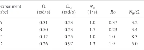
hours. Table I shows a selection of typical experiment pa-rameters. Of the four experiments shown, the diffusive insta-bility was observed to occuronly in experiments A and B. These four experiments will henceforth be used to illustrate our discussion throughout. Of course, the mechanism for McIntyre’s viscous overturning instability is the same for all ␴⬎1. However, we did not attempt to vary␴ in our experi-ments. It should be noted, however, that in the experiments by Baker13 and Calman,14 the Schmidt number was varied between 310⬍␴⬍1800, and the instability was observed to form within this range 共provided, of course, the necessary instability criteria was satisfied兲.

B. Observations

Before discussing the instability formation, we first de-scribe how the required flow conditions are established. At t= 0 the disk motion is initiated, with the container sidewalls remaining stationary relative to the rotating frame. The re-sulting spin-up processes thereafter establish two regions of flow, denoted I and II, which are shown schematically in Fig. 2; the left-hand and right-hand halves of the diagram depict the early and later stages of the flow development, respectively.

After several rotation periods, a thin boundary layer is established above the disk surface wherein the fluid is accel-erated and spun-up by the action of viscous stresses. No longer stationary relative to the rotating frame, the boundary-layer fluid is forced radially outward by Coriolis acceleration and replaced with lighter fluid from the overlying interior by Ekman suction.22,23 On encountering the container sidewall, the radial flux is forced upward into the lighter interior, es-tablishing a local adverse vertical density gradient which overturns the fluid, forming a secondary meridional circula-tion. Initially, therefore, the spun-up fluid forms the frontal region,I, confined to the lower corners of the container关see Fig. 2共a兲兴 consisting of the heaviest fluid, originally posi-tioned above the disk. The vertical extent of the front is determined by the relative strength of the background strati-fication共N/⍀兲.

[image:6.612.316.560.84.169.2]

RegionIIconsists of the interior fluid above the bound-ary layer and region I. Henceforth,BB

⬘

will be used to de-note the interface between regions I andII, while AB

⬘

will denote the early stage interface between the boundary layer and regionII关as shown in Fig.2共a兲兴. Vertical Ekman suction increases cyclonic vorticity inside regionII共by stretching the background vorticity兲, thereby generating zonal velocity, the TABLE I. A selection of four experiments chosen to illustrate the parameter ranges in which the diffusive instability was observed共A and B兲and was not observed共C and D兲.

Experiment label

⍀ 共rad/s兲

⍀d 共rad/s兲

N0

共1/s兲 Ro N0/⍀

A 0.31 0.23 1.0 0.37 3.2 B 0.50 0.23 1.7 0.23 3.4 C 0.12 0.25 1.0 1.0 8.3 D 0.26 0.97 1.3 1.9 5.0

(7)

magnitude of which decreases with heightz, with the fluid furthest above the disk remaining largely unaffected. A sche-matic illustration of the induced zonal shear flow established in regionIIis shown in Fig.2共c兲. Furthermore, directly above AB

⬘

, Ekman suction acts to deform the initial, near-planar isopycnals downward, whereas above the developing corner front共region I兲 they are forced upward, as depicted in Fig. 2共a兲. Again, far above the disk surface, the isopycnals remain largely unaffected.

The features described above are readily identified in Figs.3 and 4, which show共or include兲 data obtained from experiment A after n=共⍀/2␲兲t= 9 rotation periods 共t⬇3 min兲. In particular, note the direction in which the density profiles are deformed relative to the initial linear state共Fig.3兲, with the initial formation of regionIevident at r/R= 0.9, for z/Hⱕ0.15 共below which the fluid is well-mixed兲. Also note the form of the axisymmetric zonal shear flow¯v共r,z,t兲, with¯vz⬍0 and the no-slip condition establish-ing a region in which¯vr⬍0 near the tank sidewalls共Fig.4兲. The processes described above continue, causing region Ito expand radially inward as it is supplied共via the boundary layer兲 with fluid from region II, the density of which is gradually decreasing with time. In doing so, the contact area AB

⬘

between the boundary layer and regionII gets progres-sively smaller, thereby reducing the radial flux and the ver-tical Ekman suction on region II. Eventually, region I ex-pands to cover the area above disk surface共i.e.,AB

⬘

= 0兲, as depicted in Fig.2共b兲. At this point, the direct supply of inte-rior fluid to regionIvia the disk boundary layer共and Ekman suction兲 is effectively switched off, whereafter lighter fluid from regionIIis entrained directly through the interfaceBB

⬘

by diffusion, reducing the rate at which the fluid in regionII is spun-up. In experiment A, this event occurs aftern⬇120 rotation periods 共t⬇42 min兲. After this time, the interior

region IIflow is essentially quasisteady, while the interface BB

⬘

migrates slowly upward through the fluid. The small velocity difference between the disk surface and the fluid belowBB

⬘

maintains a weak, secondary meridional circula-tion in regionI.

The later stages of the flow development for experiment A are shown in Figs.4 and5, aftern= 720 rotation periods 共t⬇4 hours兲. The interface BB

⬘

is now clearly evident in each density profile atz/H⬇0.25, below which the fluid is essentially well-mixed and largely spun-up关see Fig.4共d兲兴. It is worth noting here that when Experiment A was terminated after 24 hours 共n= 4125兲, the interface BB

⬘

had only ad-vanced to a position at z/H⬇0.45. Also note in Fig.4 the marked decrease in the rate at which the fluid in regionIIis spun-up during the period betweenn= 120 and 720, in com-parison with the rate observed during the early stages be-tweenn= 9 and 120, when the Ekman dynamics are preva-lent. This quasisteady nature of the interior flow is further confirmed by Fig.6, showing the temporal development of the zonal flow field ¯v共r,z,t兲 at the mid-disk radius r/R = 0.5.

In Figs.5共a兲and5共c兲, the regular steplike perturbations to the near-linear background density stratification共in region II兲 are the manifestation of the axisymmetric viscous over-turning instability identified by McIntyre.3We now focus our attention on region II and describe how this density micro-structure is observed to form. For further details regarding the dynamics leading to the formation of regionI, the reader is referred to related numerical and experimental studies.9–12 In Sec. II we presented the linear theory to describe this diffusive instability mechanism. Recall that a basic require-ment of this theory was for the background flow to be in the balanced state represented by Eq.共2兲. Indeed, over the range of conditions considered in this article, the instability was 0 0 0 0 0 0 0 0 0 0 0 0 0 0 0 0 0 0

1 1 1 1 1 1 1 1 1 1 1 1 1 1 1 1 1 1

0

1

density probes (on vertical

traverse)

REGION II

REGION I

rotating disk

(a) Initial stages (b) Later stages

Ω+Ωd

Ekman suction isopycnals

B

B’ A

z

_

H Ω r R/

B’

B

REGION II:zonal shear flow; density step structures observed

REGION I:spun-up, well-mixed fluid

(c) zonal shear flow z

_

H

r R/ v _

(r,z,t)

0

[image:7.612.117.498.54.281.2]

1

FIG. 2. Schematic showing the important flow characteristics leading to the development of the flow regionsIandII共see text for description兲. The left-hand and right-hand halves of the diagram show the early and later stages of the flow development. The inset共c兲illustrates the form of the axisymmetric zonal shear flow¯v共r,z,t兲observed in regionII.

(8)

observed to form only in regions of the interior flow which eventually satisfy this condition, following the initial period of共notably兲unsteady flow as the fluid interior adjusts to the onset of disk rotation. Moreover, the staircase density micro-structure was observed to form only at timesafterthe local flow had reached this balanced state. This is demonstrated by Fig.7 which shows, for the four experiments listed in Table I, the times at which the flow is共or is not兲in balance; here, Eq. 共2兲, in slightly rearranged form, is represented by the horizontal broken line. In all cases, the data shown are taken from the interior pointr/D= 0.5,z/H= 0.52. Recall the mi-crostructure was observed to form in experiments A and B 共represented by ⫻ and +兲, in which Ro is small, but not in experiments C and D 共represented by 쎲 and 䊊兲 where Roⱖ1. Consider first experiments A and B. The data for these two experiments 共⫻, +兲 show that the flow 共at this point兲reaches the balanced state aftern⬇150 disk rotations. Note, however, in both experiments the density step struc-tures do not become fully formed at this point until much later, i.e., for experiment A aftern⬇720共as shown in Fig.5兲. Conversely, the data for experiments C and D 共쎲 and 䊊兲 show clearly that at no time is either flow in balance at r/D= 0.5, z/H= 0.52. Experiment C simply corresponds to the case of weak background rotation 共with Ro= 1.0 and

⍀⬇0.1 rad/s兲, in which the Coriolis effects are not domi-nant. Experiment D, in addition, corresponds to the case of relatively strong forcing of the flow by the disk motion共with Ro= 1.9 and⍀d⬇1 rad/s兲, in which case previous studies10

have shown共using a setup similar to the one described here兲 that the induced flow is three-dimensional, exhibiting signifi-cant secondary azimuthal wavelike modes.

The density perturbations first develop in the lower re-gion ofII共above the interfaceBB

⬘

兲; Fig.8shows a sequence of shadowgraph images, taken at various times throughout experiment A. Initially, two共or three兲step structures appear in the form of axisymmetric curved horizontal sheets. As time progresses and the fluid is gradually spun-up, more of the interior region II is destabilized resulting in additional step structures forming further above the interfaceBB

⬘

. Once fully formed, the steplike perturbations have a remarkably regular wavelength and remain robust until they are either entrained through the slowly advancing interfaceBB

⬘

, or the table or disk rotation is terminated, and the fluid is spun down. Notably, the step structures do not appear to be unduly affected by the vertical motion of the traversing conductivity probes.

It should be noted that the shadowgraph images can be somewhat misleading, due to the depth-integrated view

(a)

n

= 9 (

t

~

_{~ 3 min)}

0.9

0.2

z

_

H

-0.8 0 0.8

(

r

cos

θ

)/

R

(b)

/ = 0

r R

0 1

z

_

H

1.00 1.02

ρ

/

ρ

1

(c)

/ = 0.5

r R

0 1

z

_

H

1.00 1.02

ρ

/

ρ

1

(d)

/ = 0.9

r R

0 1

z

_

H

1.00 1.02

[image:8.612.103.513.47.402.2]

ρ

/

ρ

1

FIG. 3. Measurements obtained from experiment A aftern=共⍀/2␲兲t= 9 rotation periods.共a兲A shadowgraph image obtained during the early stages of the flow development; the homogeneous region shows where the fluid remains unperturbed and共essentially兲linearly stratified.关共b兲–共d兲兴A set of measured density profiles obtained at this time, where␳1denotes the value of␳s共r,z兲atz= 0.9H; corresponding radial locations共r/R= 0 , 0.5, 0.9兲are indicated. The initial

density profile for the solid rotation state共t⬍0兲is shown by the broken lines.

(9)

through the side of the tank. That is, in Figs.5共a兲and8, the microstructure appears to take the form of axisymmetric, saucer-shaped sheets, extending horizontally across the cyl-inder. This is not the case. The density measurements show that around the stagnant central axis共r= 0兲 the background density field remains unperturbed and essentially linear, as shown by Fig.5共b兲. Here, the necessary conditions for the onset of instability are not satisfied in this stagnant region. 共This ring-shaped structure of the sheets was also identified by Calman.14兲However, Fig.5共b兲does show the presence of a weak and smeared density step structure in the interior regionII, atr= 0. These structures were observed in the axial density profiles only during the later stages of the experiment 共in this case,n= 720, i.e., after 4 hours兲, and several hours after the step structures have formed in the midradius pro-files. This manifestation of the density microstructure at r = 0 is likely to be due to共neglected兲nonlinear effects.

Before turning to the stability question, we need to ad-dress what is an interesting consequence of the data shown in Fig.7. Linear spin-up theory共see Refs.2,5, and6, for ex-ample兲 indicates that in the early stages of spin-up, the Ek-man flux isO共E1/2兲and the meridional velocity components in the fluid interior are alsoO共E1/2兲 as a result. That being the case, the terms in the azimuthal vorticity equation not shown in Eq. 共2兲 are very small. Thus, it seems surprising that the data for experiments A and B in Fig.7 show a large

deviation from the balanced state given by Eq.共2兲during the initial stages共betweenn= 0 and 150 rotation periods兲of the flow development. The authors are grateful to an anonymous referee for making this observation. We consider that the reasons for this anomaly go to the inherent nonlinearity of the experiments reported here, for whichRo=O共1兲. There is no existing theory for this nonlinear regime, so the orderings are unclear. There are two difficulties. First, the Ekman layer itself is nonlinear, which means that there is no local Ekman suction law analogous to the familiar linear one.24The non-local character is critical, since now the layer develops from center to rim, with the entire structure nonlinearly coupled to the flow above it. Second, there is the question of the corner eruption of Ekman fluid, a prominent and crucial feature of linear spin-up, first noted by Walin.5 There is no reason to expect that such an eruption in the nonlinear regime re-sembles closely that in the linear flow—there will be strong coupling of the corner eruption with the rest of the boundary layer, likely leading to unpredictablea prioriorderings of the interior flow.共For an example of how complex that coupling can be, the reader is referred to Belcheret al.25 and related papers.兲In summary, the clear ordering arguments in linear spin-up depend crucially on the local Ekman suction law; in the absence of such simplified dynamics, the orderings of the interior flow cannot be accomplished with any confidence. In fact, the data of Fig.7suggest precisely that there are interior

(a) /

z H

= 0.72

n= 9 n= 120 n= 720

0 1

r R

vR

/

_

Ω

d

(b) /

z H

= 0.52

n= 9 n= 120 n= 720

0 1

r R

vR

/

_

Ω

d

(c) /

z H

= 0.32

n= 9 n= 120 n= 720

0 1

r R

vR

/

_

Ω

d

(d) /

z H

= 0.12

n= 9 n= 120 n= 720

0 1

r R

vR

/

_

[image:9.612.104.509.49.381.2]

Ω

d

FIG. 4. Experiment A: Measurements of zonal velocity fieldv¯_共r,z,t兲at heightsz/H= 0.12, 0.32, 0.52, 0.72; three sets of measurements are included in each plot, obtained aftern=共⍀/2␲兲t= 9, 120, and 720 rotation periods, as indicated. Error bars are provided in then= 9 measurements共every fifth data point兲to indicate the typical variation. A similar degree of variation was observed in each of the data. The broken line shows the corresponding disk speed共r⍀d兲at each radial position, and therefore represents the limiting spun-up state.

(10)

meridional velocities共during the early stages兲that are much larger than O共E1/2兲, although the detailed measurements of the meridional plane velocity fields that are necessary to con-firm this behavior were excluded from consideration in our experiments. While further experiments designed to investi-gate meridional flow fields are of merit in this regard, we emphasize here that the initial stage of the spin-up process has no real relevance to the core stability analysis we present

in this paper. For that reason, we focus henceforth on the later stages when the flow is quasisteady and the instability occurs. Before doing so, however, we note for completeness that an increase in effective viscosity of the fluid共because of

(a)

B’ B

n

= 720 (

t

~

_{~ 4 hrs)}

0.9

0.2

z

_

H

-0.8 0 0.8

(

r

cos

θ

)/

R

(b)

/ = 0

r R

0 1

z

_

H

1.00 1.02

ρ

/

ρ

1

(c)

/ = 0.5

r R

0 1

z

_

H

1.00 1.02

ρ

/

ρ

1

(d)

/ = 0.9

r R

0 1

z

_

H

1.00 1.02

[image:10.612.102.511.47.400.2]

ρ

/

ρ

1

FIG. 5. Experiment A, as in Fig.3, except thatn=共⍀/2␲兲t= 720. At this time, regionIis fully established across the disk surface, withBB⬘atz/H⬇0.25.

0 200 400 600 800

0 1

z H

/ = 0.12

/ = 0.32

/ = 0.52

/ = 0.72

n

t

vr

= ( / 2 )

/

_

d

Ω

π

FIG. 6. Experiment A: Plot showing the temporal development of the zonal flow field atr/R= 0.5. Data are shown for each of the sample heights

共as indicated兲, with the error bars showing the corresponding rms variation.

0 200 400 600 800 1000

0 0.5 1.0 1.5

n

t

v

rv

gr

s

= ( /2 )

2 _

(/

_

+)

__

zr

Ω

[image:10.612.317.557.507.694.2]

π

FIG. 7. Plot showing when the four experiments listed in TableIare共or are not兲 in the balanced state represented by Eq. 共2兲. Note the vertical axis shows the rearranged form −2共⍀r+v¯兲¯vz/grs¯r= 1 of Eq.共2兲, so that balance

is represented by the horizontal broken line. The data shown are from ex-periments A共⫻兲, B共+兲, C共쎲兲, and D共䊊兲, all taken from the interior point

r=r0= 0.5Randz=z0= 0.52H.

[image:10.612.56.295.551.724.2]

(11)

the presence of tracer particles兲 has been invoked by the referee as a possible explanation for the imbalance aspect of the initial state behavior outlined above. 共Recall that such particles were not present in the experiments used to obtain the density measurements.兲 However, the viscosity correc-tion in a dilute suspension of small particles is known26to be a multiplier of共1 + 5␣/2兲, where ␣ is the concentration of particles by volume. In our experiments, ␣ is always less than 5⫻10−4_{, and so the viscosity correction is clearly}

neg-ligible for these conditions.

We conclude this discussion by noting that the initial period of rotating-stratified spin-up problems, forRo=O共1兲, is currently not well understood and requires further detailed study.

IV. LARGE-␴CASE

It turns out that one may use asymptotic techniques to considerable advantage to obtain relatively simple results for the most unstable mode. Not only is␴large for the water-salt system, but the numerical values of⌰1and⌰2are generally

large and negative in this series of experiments. Hence, we construct asymptotic solutions for ␴→⬁, simultaneously with⌰₁,⌰₂→−⬁.

If 兩⌰₁兩,兩⌰₂兩Ⰷ1, and are both negative 共as they are in the experiments兲, then Eq. 共10兲, written here again for convenience,

共␻+k2兲2共␻+k2/␴兲+共I+G兲␻+共I/␴+G兲k2= 0, 共16兲 and the fact that I and G are both positive for large and negative ⌰1,⌰2 indicate that there can be no positive real

root for␻, since all of the terms are positive. However, we know from McIntyre3 that the instability that arises at large ⌰1⌰2 is monotonic, and it is evident from the experiments

that⌰1⌰2 is in fact quite large. The only way that Eq.共16兲

might exhibit a positive real root is if the multiplier of either the large⌰1 or ⌰2 terms inI or G is small, that is, either

cos␾or sin␾must be small, thereby making eitherI or G negative. So,␾must be near 0 or␲/2. It turns out that the latter case is the one that leads to instability.

A. Stability for␾=O_„1_…

If⌰1,⌰2→−⬁,␴→⬁, then Eq.共16兲becomes, to

lead-ing order,

共␻+k2_兲2_␻₋_共_⌰

1sin2␾+⌰2cos2␾兲␻−⌰2k2cos2␾

= 0, 共17兲

so long as␾is such that neither the sine or cosine is small. We have dropped for the moment the 1/␴terms, since they contribute higher-order corrections to what follows. Then, using the largeness of the three parameters, and assuming that␻=O共1兲, we get to leading order the stable root

␻⬃−

冉

⌰2cos

2_␾

⌰1sin2␾+⌰2cos2␾

冊

k2+O

冉

1 ⌰1

, 1 ⌰2

,1 ␴

冊

.

共18兲

Certainly, an asymptotic solution for␻depends on the rela-tive orderings of the three large parameters in this problem, ⌰1, ⌰2, and ␴. Nonetheless, a more formal approach than

what is presented here shows that, in order to obtain Eq.共18兲 from Eq. 共17兲, we need require only that ⌰1=O共⌰2兲 and

1/␴=o共1兲.

The other two roots correspond to large values of␻, and scaling␻with

冑−

⌰₁, construction of a two-term series gives the damped, oscillatory modes

␻⬃ ⫾i冑−⌰1

冉

sin2␾+

⌰2

⌰1

cos2␾

冊

1/2

−k

2

冉

2⌰₁sin2␾+⌰₂cos2␾ ⌰1sin2␾+⌰2cos2␾

冊

, 共19兲

for⌰1,⌰2→−⬁. Once again, since␴Ⰷ1, the corrections to

this expression are higher order.

So, even though the three roots are of differing scales at large共−⌰1兲, none of them leads to an instability of this flow.

We now turn to an analysis of the solutions for␻when␾is near␲/2.

-0.8 0 0.8

0.2 0.9

-0.8 0 0.8

0.2 0.9

-0.8 0 0.8

0.2 0.9

r

R

z

H

n

t

r

R

n

t

r

R

n

t

_

( cos )/

(a) = 80 ( ~~28 min)

( cos )/

(b) = 220 ( ~~1.3 hrs)

( cos )/

(c) = 430 ( ~~2.5 hrs)

[image:11.612.68.544.50.186.2]

θ

FIG. 8. Experiment A: Sequence of shadowgraph images illustrating the development of the density microstructure in regionII.

(12)

B. Instability for␾È␲/ 2

To examine this case, we write

␾=␲ 2 +␾

˜_, _兩_␾˜_兩_Ⰶ_1,

so the parameters that occur in the Eq.共16兲take the approxi-mate form

I⬃−␾˜ −⌰1, G⬃−␾˜ −⌰2␾˜2, 共20兲

taking ␾˜ to be small and ⌰1 and ⌰2 large and negative.

Substituting into Eq. 共16兲then gives the approximate poly-nomial in this regime,

共␻+k2兲2共␻+k2/␴兲−共2␾˜ +⌰1+⌰2␾˜2兲␻

−关␾˜ +⌰2␾˜2+共˜␾+⌰1兲/␴兴k2= 0. 共21兲

Retaining only the dominant terms in the asymptotic limits described above, and fork=O共1兲, this equation becomes

共␻+k2兲2␻−⌰1␻−共␾˜+⌰2␾˜2+⌰1/␴兲k2= 0. 共22兲

Then, so long as ␻ is not large, we get the approximate solution

␻⬃−

冉

␾ ˜₊_⌰

2␾˜2+⌰1/␴

⌰1

冊

k2+O

冉

1 ␴⌰1

冊

. 共23兲

关The two oscillatory roots, Eq.共19兲, do not alter dramatically in this regime from those results given above, since putting ␾=␲/2 in that equation clearly does not invalidate those asymptotics.兴 Now, clearly for ␾˜ sufficiently large, ␻ goes like −k2_{, indicating stability. Since the denominator is always}

negative, the requirement for instability becomes

␾ ˜ ₊_⌰

2␾˜2+⌰1/␴⬎0. 共24兲

This polynomial is positive provided ␾˜ lies between two roots, that is,

␾ ˜

−⬍␾˜⬍␾˜+,

where

␾ ˜

⫾= − 1 2⌰2

⫾

冑

1 4⌰₂2−

⌰1

␴⌰2

.

This range shrinks to zero when the square root vanishes. Thus, for a finite range of␾˜ that obeys criterion 共24兲, and hence leads to共monotonic兲instability, we require

⌰1⌰2⬍

␴

4, k=O共1兲. 共25兲

This result agrees with the large-␴limit of McIntyre’s result, Eq. 共13兲. Before modifying this result for large k, we note that␾˜ in the critical range of Eq.共25兲is of order 1/⌰2, and

is therefore small as initially assumed. Again, formal asymp-totics show that result 共23兲 is asymptotically valid for 兩⌰1兩→⬁ provided that ⌰2=O共⌰1兲, but also now that

␴=O共⌰1⌰2兲, which is consistent with our experiments.

C. The instability at largekfor␾È␲/ 2

We have found an instability that occurs near ␾=␲/2 whose growth rate is proportional to the square of the wave number, and so grows to larger values askincreases. On the other hand, it is immediately obvious forksufficiently large that all solutions to Eq. 共16兲 are stable, that is, R兵␻其⬍0. Therefore, at some intermediate value of kwhich evidently must be large,␻passes through zero. We seek in this section to examine the instability in that range of k. We note from Eq.共23兲 that ␻scales withk2_/_␴_{, but from Eq.} _共₂₁_兲_{, on the}

other hand, since␻ is smaller than k2_{, we obtain a scaling}

␻⬃k6_/_共_⌰

1␴兲. Balancing these gives k⬃共−⌰1兲1/4 if we take

␴=O共⌰1⌰2兲as above. Then,␻is of order共−⌰1兲−3/2. Hence,

we now write

k=共−⌰1兲1/4␭, ␻=

共−⌰1兲1/2

␴ ⍀. 共26兲

Substitution into Eq.共21兲gives the leading-order result

⍀= − ␭

2

1 +␭4

冋

␭

4₊ ␴

⌰1⌰2

冉

⌿+⌿2+⌰1⌰2 ␴

冊

册

+O

冉

1 ⌰1

冊

, 共27兲

for ␾˜=⌿/⌰2. The instability criterion 共25兲 is recovered if

␭2_Ⰶ_1.

Since the result共23兲is wholly contained in Eq.共27兲, we can compute ␻ versus k for a given value of ⌿ from Eq. 共27兲. Parametric restrictions here are those of the foregoing k=O共1兲 discussion. Typical results are shown in Fig. 9 for both stable and unstable cases. We note that in Eq.共23兲 the growth rate is order 1/␴, when k=O共1兲. However, in this regime, the growth rate is order共−⌰1兲1/2/␴, much larger, and

so maximum growth rates occur fork=O关共−⌰1兲1/4兴.

0 0.4 0.8 1.2 1.6 2.0

-4 -3 -2 -1 0 1

k

_

/(

)

/(

)

1 1/4

1

1/2

Θ

[image:12.612.319.556.50.239.2]

σω

FIG. 9.␻vskfor three values of⌰1⌰2/␴and with⌿= −1/2. The cases shown are: ⌰1⌰2/␴= 0.1 共solid line兲, ⌰1⌰2/␴= 0.2 共dashed line兲, and

⌰1⌰2/␴= 0.5 共dotted-dashed line兲. Recall from Eq. 共25兲 that monotonic instability occurs when⌰1⌰2/␴⬍0.25.

(13)

Clearly, the maximum growth rate arises when both ⌿ and␭derivatives of⍀vanish. That occurs at⌿m= −1/2 and, after solving a quadratic for␭4_{, at}

␭m4

=⌽− 3 +

冑

共1 −⌽兲共9 −⌽兲

2 , 共28兲

where

⌽⬅

冉

1 − ␴ 4⌰1⌰2

冊

. 共29兲

Substitution into Eq.共27兲 gives this maximum value of the growth rate as

␻m⬃共−⌰1兲1/2

␴

冋

3 − 3⌽−

冑

共1 −⌽兲共9 −⌽兲 ⌽− 1 +

冑

共1 −⌽兲共9 −⌽兲

册

⫻

冋

⌽− 3 +

冑

共1 −⌽兲共9 −⌽兲

2

册

1/2

. 共30兲

The associated wave number is given by

km⬃

再

− ⌰1

2 关⌽− 3 +

冑

共1 −⌽兲共9 −⌽兲兴

冎

1/4

, 共31兲

which is real only for⌽⬍0, and that occurs if Eq.共25兲 is satisfied.

To summarize then, the most unstable mode of form共9兲 is

exp

冋

i共−⌰1兲1/4␭m

冉

y+

x 2⌰2

冊

+␻m␶

册

, 共32兲

where this asymptotic result is valid for

⌰1,⌰2→−⬁ and ␴=O共⌰1⌰2兲. 共33兲

In dimensional form, the characteristic vertical length scale 共L兲and time scale共T兲for this most unstable mode are given by

L=2␲ km

冉

␯2

g␤¯s_r0

冊

1/4

and T=2␲ ␻m

冉

1 g␤¯s_r0

冊

1/2

. 共34兲

D. Comparison with experiment

Theoretical predictions were compared with measure-ments from the experiment data atr₀/R= 0.5,z₀/H= 0.52. At this interior point, the measured density and zonal velocity fields共and associated gradients兲were not unduly affected by the advancing frontal region, or by the tank sidewall. More-over, this point provided a period of at least 1 hour before the flow became unstable, allowing the corresponding onset time for the instability to be determined. This is illustrated by Fig. 10, which shows⌰1⌰2 plotted againstn for experiments A

and B. Also shown are the conditions for monotonic and oscillatory instability; the latter is obtained directly from Eq. 共14兲, by taking the␴Ⰷ1 limit.共Note that in all experiments considered here, and as illustrated in Fig.10, the condition for oscillatory modes was never satisfied.兲When Figs.7and 10are compared, we see that it takes aroundn= 200 rotation

periods for the flow in experiments A and B to reach approxi-mate gradient wind balance 共i.e., about 70 and 40 min, respectively兲.

It is possible to compute ⌰1⌰2 from linear, spin-up

theory, of the kind reviewed elsewhere,2 and then compare with the experimentally obtained product shown in Fig.10. However, there is a serious difficulty with such a compari-son: the linear spin-up theory requires RoⰆ1, and in the initial stages of the spin-up, due to the corner eruption, RoⰆE1/2, whereE=␯/⍀H2is the Ekman number共which is about 5⫻10−5 in our experiments兲. In fact, here, RoⰇE1/2. Of all the small parameters that are relevant to such an analy-sis共viz.,Ro,E1/2,␴−1兲, the Rossby number is by far the larg-est. After temporal adjustments have occurred, and for the case for which␴RoⰇ1共as in these experiments兲, though the gradient wind balance remains approximately linear, the equations for the zonal velocity component and the density perturbation are inherently nonlinear. Salinity perturbations near the boundary, in a layer of width E1/2_/_共_␴_Ro_兲1/3_{, drive}

similar perturbations in the thicker共E1/2_兲 _{Ekman layer, and}

that induces a nonzero salinity perturbation in the interior. We denote byLexpthe height共or wavelength兲of the fully

developed density step structure observed in the experi-ments, measured directly from the midradii density profiles at the point共r₀,z₀兲. This step height was compared with the corresponding vertical perturbation length scaleL predicted by the theory. The results for experiments A and B are given in TableII. Once fully developed, the height of the density

0 200 400 600 800 1000 1200

0 100 200 300 400 500

n

= ( /2 )

t

12

Ω

ΘΘ

π

Θ Θ Θ Θ

1 2 1 2

= 9/8