Influence of Lateral Transshipment Policy on Supply Chain Performance: A Stochastic Demand Case

doi:10.4236/ib.2010.21009 Published Online March 2010 (http://www.SciRP.org/journal/ib)

Influence of Lateral Transshipment Policy on

Supply Chain Performance: A Stochastic Demand

Case

Jingxian Chen1_{, Jianxin Lu}2

1_{School of Business, Nantong University, Nantong, China;} 2_{Institute of Logistics Engineering, Nantong University, Nantong, China.}

Email: carl.jxchen@hotmail.com, jxchen@ntu.edu.cn

Received September 14th_{, 2009; revised October 25}th_{, 2009; accepted December 2}nd_{, 2009.}

ABSTRACT

Considering the supply chain consists of one supplier and two retailers, we construct the system’s dynamic models which face stochastic demand in the case of non-lateral transshipment (NLT), unidirectional lateral transshipment (ULT) and bidirectional lateral transshipment (BLT). Numerical example simulation experiments of these models were run on Venple. We adopt customer demand satisfaction rate and total inventory as performance indicators of supply chain. Through the comparative of the simulation results with the NLT policy, we analyze the influence of ULT policy and BLT policy on system performance. It shows that, if retailers face the same random distribution demand, lateral transshipment policy can effectively improve the performance of supply chain system; if the retailers face different ran-dom distribution demand, lateral transshipment policy cannot effectively improve the performance of supply chain sys-tems, even reduce system’s customer demand satisfaction rate, and increase system inventory variation.

Keywords: Supply Chain, Inventory System, Lateral Transshipment, Performance

1. Introduction

Lateral transshipment, an important inventory replen-ishment policy, has gained a common concern of the academics and business managers in recent years. There are numerous researches about this issue. Lateral trans-shipment is defined as the redistribution of stock from retailers with stock on hand to retailers that cannot meet customer demands or to retailers that expect significant losses due to high risk [1]. The early pioneering work of Krishnan and Rao [2] examine a periodic review policy in a single-echelon, single-periodic setting [2]. Robinson [3] extends the research to a multi-period case, and es-tablishes the system’s lateral transshipment model [3]. The emergency lateral transshipment model of repairable product was analyzed by Lee [4] for the two-echelon inventory system case [4]. Axsäter [5] studies the emer-gency lateral transshipment problem of the multi-level repairable product inventory system, and gets some in-teresting conclusions different from Lee’s [5]. Archibald et al. [6] develop a lateral transshipment model among the multi-retailer based on Markov decision-making methods [6]. Grahovac and Chakravarty [7] limit the research object to low demanded expensive product and

multiple retail points [15]. Huo and Li [16] develop batch ordering policy in a single-echelon, multi-location trans-shipment inventory system [16]. Li et al. [17] study in-ventory management model of the cluster supply chain system with the existence of emergency lateral trans-shipment [17].

Most of the papers above dealing with transshipment assume that lateral transshipment already exists in system. However, lateral transshipment will make the problem complicate and tend to be very difficult to analyze ana-lytically, especially BLT [18]. Hence, will lateral trans-shipment really need? This paper handles this problem from the performance measurement point. We consider one supply chain system consists of one supplier and two retailers, allowing a retailer transship from the other one for inventory replenishment besides order from supplier. System’s models were developed by system dynamics assume that all the members use the order-up-to policy, and numerical experiment was run on Venple platform.

The paper is organized as follows: in Section 2, the models with lateral transshipment were developed, as well as without lateral transshipment. The accuracy of the model is tested against simulation in Section 3; Sec-tion 4 deals with the influence of ULT and BLT. The conclusion of this paper was presented in Section 5.

2. Model Description

We consider two retailers facing independent stochastic customer demand and one supplier (Figure 1). Without lateral transshipment, retailers order from suppliers to replenish inventory in case of stock out. In order to re-spond to customer demand quickly, they can use lateral transshipment policy besides order from the supplier, which means they replenish inventory from the other one if there exist surplus stock on hand.

2.1 Model Assumption

Development of the model needs the following assump-tions.

 Customer1 and Customer2 face independent stochas-tic demand;

 Both retailers adopt order-up-to policy, the ordering

period is constant;

 Lateral transshipments take no time;

 Transshipments take place when there are surplus stocks. That is, if retailer 1 needs transshipment from retailer 2, retailer 2 only transships the redundant stock. 2.2 System Model

As a modeling and simulation technology, system dy-namics has a wide range of applications since its birth, especially in dealing with long-term, chronic, dynamic management problems [19]. Forrester [20] applies sys-tem dynamics in industrial business management, ad-dressing issues such as fluctuations in production and employees, instability of market shares and market growth [20]. Logistics and Supply Chain Management is an important area of System Dynamics. Sterman [21]de-signs the well-known beer game by System Dynamics, and carries out detailed analysis on feedback loops, nonlinear, time-delay and management behavior in the system [21]. Diseny et al. [22] analyze VMI in transport operation by system dynamics [22]. Marquez [23] estab-lishes a model for measuring financial and operational performance in the supply chain based on System Dy-namics [23], and so on.

Generally speaking, a complete system dynamics model usually consists of three parts: model variables, causal loop diagrams and mathematical description. We analyze the three part of model in turn as follows.

2.2.1 Model Variables

The structure of a system dynamics model contains stock, smoothed stock, flow rate, auxiliary variables and con-stants. Stock variables are used to describe the cumula-tive effect of the system. Smoothed stock variables are the expected values of specific variables obtained by exponential smoothing techniques. Flow rate describes the rate of the cumulative effect of the system. Auxiliary variables are the middle variables which express the de-cision-making process. Constants change little or rela-tively do not change during the study period. The fun-damental notations of the model are following:

Supplier

Retailer 1

Retailer 2

Customer1

[image:2.595.136.462.598.688.2]

Customer2

Figure 1.2-echelon supply chain. Filled arrows represent the flow of regular replenishments while dashed arrows represent

Nomenclature

Indices 2 , 1 ,i

i index for retailers

2 , 1 ,j

j index for retailers

Stock Variables

SI inventory of supplier IRi inventory of retailer i

Smoothed Stock Variables

AOQRi average order quantity of retailer i ASRRi average sales rate of retailer i Flow Rate Variables

SRTRi shipment rate to retailer i ORRi order rate of retailer i ORS order rate of supplier SRRi sales rate of retailer i LTij lateral transshipment from retailer to retailer i j

Auxiliary Variables and Constants

DICTS desired inventory cover time of supplier

DIS desired inventory supplier IGS inventory gap of supplier

IARS inventory gap of supplier IATS inventory adjustment rate of supplier

OQS order quantity of supplier ODTS order delay time of supplier

ASRSTRi average sales rate smooth time of retailer i

ODTRi order delay time of retailer i OQRi order quantity of retailer i

AQRSTRi average order quantity smooth time of retailer i

IGRi inventory gap of retailer i DIRi desired inventory of retailer i

DICTRi desired inventory cover time of retailer i IARRi inventory adjustment rate of retailer i

IATRi inventory adjustment time of retailer i CDRi customer demand of retailer i

CSRRi customer demand satisfaction rate of retailer i

TI total inventory.

2.2.2 Causal Loop Diagrams

Causal loop diagram is a tool that expresses the structure of the system, playing an extremely important role in system dynamics. There are two reasons for that. First, during model development, they serve as preliminary sketches of causal hypotheses and secondly, they can simplify the representation of a model.

The first step of our analysis is to capture the relation-ship among the system operations in a system dynamics manner and to construct the appropriate causal loop dia-gram. Figure 2 describes the causal loop of the supply chain without lateral transshipment.

The system structure in Figure 2 contains supplier and retailers. For the supplier, is decided by and

. is determined commonly by _OQS and . Delivery rate is determined by and . Supplier adjust inventory level by setting , together with determine . and determine , in turn, has a direct impact on

SI SRTRi

IARS

ORS SRTRi

ODTS SI

ORS

IARS

OQRi DIS IATS SI IGS IGS

OQS IRi

cided by

and an indirect impact on ORS. For retailers, is determined by ORRi and . is the delay of , delay time is . is

de-SRRi after e time etailers also adjust . DIRi is decided by

ASRRi and DICTRi. DIR jointly

deter-IGRi. Ricom nly determine

IARRi G greater 0, Retailer sent orders der quantity _OQRi is decided by

SRRi ODTRi

ORRi SRRi

is obtained f

SRTRi

IRi and rom

th R

inventory level by setting

CDRi. ASRRi

ASRSTRi.

DIRi i and and IAT

than

IRi

mo mine

to su

IGRi Ri is or . If I

ppliers,

Figure lateral t

2. Causal loop pment

ASRRi . IGRi , IARRi , and AOQSTRi determine

AOQRi. There are tw rforman s, customer satisfaction rate CSRRiand total inventory T

o pe ce variable

demand I.

[image:4.595.304.543.291.530.2] [image:4.595.57.289.322.489.2] [image:4.595.60.283.530.692.2]

CSRRi is decided by inventory IRi and customer de-mands CDRi, TI is a accumulation sum of supplier inventory SI and IRi.

Figure ribes the causal loop diagram of supply chain with ULT. 3 desc LT21 means the transshipment from tailer 2 to retailer 1. It is a flow rate variable and means that when retailer 1 out of stock, retailer 2 will replenish retailer 1 by transshipment on condition that it has sur-plus stock. L 21

re

T is decided by CDRi and IRi, and influence OQRi.

Figure 4 descr bes the causal loo gram of e sup-ply chain with BLTi . LT21 is the same as noted above.p dia th

12

LT is a flow rate variable and means that when retailer 2 is out of stock, retailer 1 will replenish retailer 2

ansshipment on condition that it has surplus stock. by tr

12

LT is decided by CDRi and IRi, and influence OQRi_.

Figure 3. Causal loop diagram of the supply chain with uni-directional lateral transshipment

Figure 4. Causal loop diagram of the supply chain with bid rectional lateral transshipment

methodology includes atical model, usually

i-2.2.3 Mathematical Description The next step of system dynamics the development of the mathem

presented as a stock-flow diagram that captures the model structure and the interrelationships among the variables. Combining mathematical description and causal loop diagram of variables, we use visual simula-tion software (Venple) to reflect the behavior of the sys-tem and provide a basis for decision-making. We analyze the mathematical description of the main variables in the system under the three cases of NLT, ULT and BLT so as to lay a good foundation for model simulation.

NLT case

 

t SI

 

t 1 dt



ORSSRTR1SRTR2



SI     (1)

 

t IR

 

t dt



ORRi SRRi

IRi  1   



(1) is the inventory dynamics equation o is the inventory dynamics equation of retailer

(2) f supplier, (2)

i.



OQRi AOQSTRi



SMOOTH

AOQRi , (3)



SRRi ASRSTRi



SMOOTH

ASRRi , (4) (3) is the average order quantity equation o

(4) is t

f retailer i, he average sales rate equation of retailer i.



SRTRi ODTRi



DELAY

ORRi 1 , ( 5)





OQS ODTS

DELAY

ORS  1 , (6)

       

 

   

  

 

 







2 1 2

1

2 1

0 0 0 0

SI OQRi and

SI OQRi OQRi

SI

SI OQRi and

SI OQRi

SI

SRTRi

(7)

    

  

 

CDRi IRi CDRi

CDRi IRi IRi

IRi SRRi 0

0 0

(8)

(5) and (6) are the order rate equations of suppliers and retailers,

ing order quantities in a given period of time. (7) is the which are the delay function of the correspond-equation of supplier shipment rate to retailers. It means when SI 0, SRTRi is 0; when SI 0 and the total order quantity



2OQRiSI, supplier can fully meet the orders of ret t rate is the order quantity of retailers OQRi; when SI0 and



2OQRiSI

1 ,

supplier partl t the ord retailers. the propor order

1

ailers, s

mee n of

hipmen

ers s, y

tio of shipmenAccording tot rate is

   

 





2

1OQRi

OQRi

SI . (8) is the sales rate equation of

CDRi, meaning that customers’ demand will be m ly, SRRiCDRi; When

CDRi IRi

retailer i. When IRi et complete 



, mean the customer de

be met partly, SRRiIRi; when ing that mand will never be met, 0

0  IRi  SRRi . DICTS OQRi

DIS

1

2  (9)

DELAY1



DIS IGS

tity equation of supplier. When IGS0 or



OQS O

ORS , DTS



(10)

SI

 (11)

IATS IGS IARS IARS and , nt. able equ uatio (12)           2

1 0 0

0 AOQRi IGS AOQRi IARS IGS OQS 





2

1 2 DICTRi , ation o n of sup

0

2

1 





AOQRi

IARS , ; When

and 0  OQS 2 1 0  IGS 0  



AOQRi

IARS ,



  2 1AOQRi IARS

OQS . (14)～(16) express the aux-iliary variables equations of retailers. (14) and (15) ex-press the desired inventory equation and the inventory gap equation of retailer . (16) is the order quantity equation of retailer . When

i

i IGRi0 or

0  ASRRi IARRi 0 

, OQS0 ; When IGRi0 and ASRRi

IARRi , OQSIARRiASRRi.

 



1 0

0orIARS AOQRi

(13) (14)

(16 ,

(9)～(13) are th f sup

plier. ( the desi plier.

(1



  2 1IRi SI

TI (17)

DICTRi ASRRi

DIRi 

IRi DIRi

IGRi  (15)

          CDRi IRi CDRi IRi CDRi IRi IRi CSSRi 1 0 0 0 (18)      

 0 0

IGRi ASRRi IARRi IGRi OQRi   0

0and IARRi ASRRi orIARRiASRRi0

)

(17) is the total inventory equation of the supply chain system. (18) is the customer demand satisfaction rate equation of the supply chain system. When IRi0,

0



CSSRi ; When 0IRiCDRi, CSSRiIRi CDRi CDRi

;

When , . is a random

variable, and it obeys a certain random distribution.

CDRi



IRi CSSRi1

DICTS ODTRiand ,ODTS AOQSTRi , IATS are , ASRSTRi consta IATRi

e auxiliary vari s s -9) is red inventory eq

0) is the order rate equation of supplier. (11) is the in-ventory gap equation of supplier. (12) is the inin-ventory adjustment rate equation of supplier. (13) is the ordquan ULT case.



 





 



               1 1 2 2 2 2 2 2 1 1 2 2 2 2 1 1 2 21 IR CDR CDR IR and CDR IR CDR IR IR CDR CDR IR and CDR IR IR CDR R LT

0 IR1CDR1or IR2CD

(19)   1 1 CDR IR CDR IR

 

1

1 and and

 

1 dt



ORR1 SRR1 LT21



1t

1t IR

IR    (20)

 

  

 

dt



ORR2 SRR2 LT21



IR2t IR2t1  (21)

21 LT

2 IGR IGR

s in th   1 ASRR  21 2 LT ariable                0 21 1 1 0 1 1 1 1 0 1 0 1 LT ASRR IARR and IGR IARR ASRR IARR or IGR

OQR LT210 (22)

             0 21 2 2 0 2 0 21 2 2 0 2 0 2 LT ASRR IARR and ASRR IARR LT ASRR IARR or

OQR (23)

(19)～(23) are the equations of v e ULT tu n,

cl



IR2CDR2

 

 CDR1IR1



, LT21CDR1IR1 ; When

si atio and the other variables which were not in-ude in the above expression are the same as the vari-ables in the NLT situation. (19) is the transshipment rate equation. When IR1CDR1 or IR2CDR2,

0 21

LT ; When IR1CDR1, IR2CDR2 and’



IR2CDR2

 

 CDR1IR1



, 21 IR1

, _{IR2CDR2 and} 1

1 CDR IR 



IR2CDR2

 

 CDR1IR1



, LT21IR2CDR2 .

0)～(23 and

their e nations are similar with NLT. BLT case.

(2 ) express the variables changed in ULT, xpla





1

CDR

LT   ;



 



 

                  2 2 CDR CDR CDR   2 2 1 1 1 1 2 1 2 2 1 1 1 1 2 2 1 2 0 12 IR CDR CDR IR and CDR IR and IR IR CDR CDR IR and CDR IR and CDR CD or LT 2 1 2 IR CDR IR IR

IR IR R1



 





 

0 2 2 1 1

21 1 1 2 2 1 1 1 1 1 1

1 1 2 2 1 1 1 1 2

IR CDR or IR CDR



2

LT CDR IR IR CDR and IR CDR and IR CDR CDR IR IR CDR IR CDR and IR CDR and IR CDR CDR IR

    _        _{     }  (25)

 

1

 

1



1 1 21 12



1t IR t dt ORR SRR LT LT

IR        (26)

 

2

 

1



2 2 21 12



2t IR t dt ORR SRR LT LT

IR       

(29)

(24)～(29) are the equations of variables in the BLT situation, and the other variables which were not in-cluded in the above expression are the same as the vari-bles in the NLT. The explanations of above equations r

ich is the validity of the set of rela-mpared with the real process. aws in system dynamics

mod-and behavior sensitivity tests [24]. Generally, the goal of extreme test lies in whether the equations a

ingful or not and whether the model condi

reasonable or not under the situation of using extreme (27)                1 1 0 1 12 21 1 1 0 12 21 1 1 0 1 0 1 ASRR IARR and IGR LT LT ASRR IARR LT LT ASRR IARR or IGR OQR   12 0 21 LT

LT (28)

              0 21 2 2 0 2 12 21 2 2 2 2 0 2 0 2 LT ASRR IARR and IGR LT LT ASRR IARR LT ASRR IARR or IGR

OQR 21LT120

a

a e the same as the ULT case, and the concrete explana-tions will be omitted.

3. Models Validation

The main criterion for system dynamics models validation is structure validity, wh

tion used in the model, as co For detection of structural fl

els, certain procedures and tests are used. These structure validity tests are grouped as direct structure tests and indi-rect structure tests. Diindi-rect structure tests involve compara-tive evaluation of each model equation against its coun-terpart in the real system (or in the relevant literature). Direct structure testing is important, yet it evolves a very qualitative, subjective process that needs comparing the forms of equations against real relationship. It is therefore, very hard to communicate to others in a quantitative and structured way. Indirect structure testing, on the other hand, is a more quantitative and structured method of testing the validity of the model structure. The two most significant and practical indirect structure tests are extreme-condition

put. Behavior sensitivity test consists of determining those parameters to which the model is highly sensitive and

re still mean- tions are still

asking if these sensitivities would make sense in the real system. If we discover certain parameters to which the model behavior is surprisingly sensitive, it may indicate a flaw in the model equations.

In view of the deficient of real data and the difficulty of gaining mass data, we only use the extreme condition test and the sensitive test in the indirect structure tests to carry on the validation for the models of this paper. We use the total inventory which is a main output of the sys-tem to confirm the performance in the extreme test and the sensitive test.

Suppose that the system is facing an extreme demand, we use Venple to test the models which are NLT, ULT and BLT, and compare the simulation results with the normal demand case. The results are shown in Figure 5. Although the total inventory becomes very big with the sharply increasing demand, the tendency is similar with the normal demand case. This indicates that the variables and the equations in the system still have effects, and the model displays a good robustness under the extreme input.

0 40 80 120 160 200 0 20000 40000 60000 80000 100000 120000 Extreme Time Tota l Inve nto ry Normal NLT 1000 1200 1400 0 200 400 600 800

0 40 80 120 160 200 0 20000 40000 60000 80000 100000 120000 Extreme 1000 1200 1400 Normal Time 0 200 400 600 800 ULT

[image:6.595.87.508.564.704.2]

0 40 80 120 160 200 0 20000 40000 60000 80000 100000 120000 BLT Extreme 1000 1200 1400 Normal Time 0 200 400 600 800 To ta l Inve ntory

Through changing the demand parameters, we use Pois-son distribution to test the models’ sensitivity, and the simulation experiment is also carried on the Venple. Fig-ure 6 presents the result that compare with the normal parameters case. We can see although fluctuation range of the total inventory is inconsistent under the two kinds of demand with different parameters, the tendency dis-plays as basically consistent. This explains that the mod-els don’t sensitively response to the parameters, and this is conducive for the model’s practical application.

4. Numerical Simulation

We employ a numerical example to examine the influ- ence of three different policies on system performance, and further analyze the simulation results and provide reasonable suggestions. In order to facilitate the numeri- cal simulation, we set the initial value of the constants,

1



AOQSTRi , ARSTRi1, DICTRi1, DICTRS2, 1



IATRi , IATS2 , ODTS2 , SI

 

0 500 ,

 

i 100

IR , T 200. Where T is the simulation time.

0 40 80 120 160 200 0

200 400 600 800 1000 1200 1400

0 40 0 200

80 120 160 200 400

600 800 1000 1200 1400

0 80 0

200 400

40 120 160 200 600

800 1000 1200 1400 NLT

[50,150]

ULT BLT

Time

T

ot

al Inv

e

nt

or

y

Time

[100,200]

[50,150]

Ti

T

ot

al Inv

e

nt

or

y

me

[100,200]

[100,200] [50,150]

or

y

T

ot

al Inv

e

nt

[image:7.595.87.511.214.700.2]

tory of two diffe mand

Figure 6. Total inven rent kinds of de

0 4 0 8 0 1 2 0 1 6 0 2 0 0 0

2 0 0 4 0 0 6 0 0 8 0 0 1 0 0 0 1 2 0 0 1 4 0 0

0 4 0 8 0 1 2 0 1 6 0 2 0 0 0

2 0 0 4 0 0 6 0 0 8 0 0 1 0 0 0 1 2 0 0 1 4 0 0

0 4 0 8 0 1 2 0 1 6 0 2 0 0 0

2 0 0 4 0 0 6 0 0 8 0 0 1 0 0 0 1 2 0 0 1 4 0 0

U L T

T

o

ta

l In

vent

o

ry

T im e N L T

N L T v s B L T

N L T v s U L T U L T v s B L T

T im e N L T B L T

T im e U L T

B L T

Figure 7. Total inventory in the same distribution demand case

4.1 Same Distribution Demand Case

[image:8.595.90.506.295.705.2]

We assume retailer i face same distribution demand that is Poisson distribution with range from 50 units to 150 units. Simulation results are shown in Figure 7, Figure 8 and Table 1.

From the simulation results, the system has the lowest total inventory in BLT case, the average size is 540.2057 units and the standard deviation is 192.2115 units; The following is that in ULT case with its mean is 546.1087 units and the standard deviation is 199.2071 units; Under the situation of NLT, the system has the largest total in-ventory, its average size is 671.9624 units and the stan-dard deviation is 215.6611 units. It can be seen, lateral transshipments policy reduces the system’s total inven-tory. However, by comparing with BLT, we can find that ULT policy reduce more total inventory. In addition,

from the standard deviation of the total inventory we can see that lateral transshipment policies make the system’s total inventory stabilized. Comparing with ULT, BLT cannot make significantly advantages. Thus it can be seen, in terms of the system's total inventory, lateral transshipment policy can effectively reduce the size and fluctuation of total inventory, but if we view from effect, little difference can be seen between BLT and ULT.

From Table 1, we see that lateral transshipment im-prove demand customer satisfaction rate. In NLT, ULT and BLT, mean of are 0.622, 0.829 and 0.772, respectively; mean are 0.630, 0.829 and 0.772, respectively. In addition, compared with the situation of NLT, customer demand satisfaction rate is more stable in lateral transshipment case. Furthermore, comparing with BLT, ULT is more efficiency in the system performance.

U

1 CSRR of CSRR2

Table 1. Simulation results in the same distribution demand case

NLT LT BLT

Mean Stdev Mean Stdev Mean Stdev

CSRR1 0.622 0.535 0.829 0.375 0.772 0.447

CSRR2 0.630 0.433 0.773

TI 671.9624 215.6611 546.1087

0.368 0.731 0.402

199.2071 540.2057 192.2115

0 4 0 8 0 1 2 0 1 6 0 2 0 0 0

2 0 0 4 0 0 6 0 0 8 0 0 1 0 0 0 1 2 0 0 1 4 0 0

0 4 0 0 2 0 0 4 0 0 6 0 0 8 0 0 1 0 0 0

8 0 1 2 0 1 6 0 2 0 0 1 2 0 0

1 4 0 0

0 4 0 8 0 1 2 0 1 6 0 2 0 0 0

2 0 0 4 0 0 6 0 0 8 0 0 1 0 0 0 1 2 0 0 1 4 0 0

To

ta

l I

n

v

entory

T im e N L T

N L T v

U L T N L T v s U L T

T im e N L T

B L T s B L T

T im e U L T

B L T U L T v s B L T

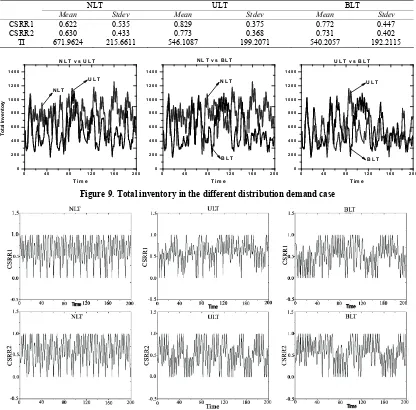
igure 9. Total inventory in the different distribution demand case F

[image:9.595.59.539.101.153.2]

Table 2. System simulation results under different distribution of the needs

NLT ULT BLT

Mean Stdev Mean Stdev Mean Stdev

CSRR1 0.633 0.426 0.604 0.377 0.552 0.447

CSRR2 0.618 0.442 0.594 0.470 0.557 0.450

TI 769.0258 229.2123 736.6729 211.6455 758.8274 240.3414

4.2 Different Distribution Demand Case

We assume retailer face different distribution demand. Retailer 1 is still subject to the Poisson distribution as described above. Retailer 2 is subject to the Normal dis-tribution with the range from 50 units to 150 units. Simulation results are shown in Figure 9, Figure 10 and Table 2.

Comparing with that in NLT situation, the system total inventory decreases in BLT and ULT cases, but slightly. In addition, viewing the standard deviation of total in-ventory in three varieties of policies, we can see that it decreases slightly in

BLT case. It shows th

with the different distribution demand case.

Table 2 we can see that lateral transshipmen decrease ustom and satisf rate in dif ferent le ecia LT. In N and BL

ean of ar 604 2, respe

d 0.557, at lateral

etailers as the research objects, this paper study

to

dema ystem,

usion of this paper, we believe that ts make the system handle inventory ses the total inventory, and improves

demand. The main reason may be that different distribu-tion demand will make ordering and replenishment be-come extremely complex. Moreover, if the retailers still use a separate order-up-to policy, lateral transshipments may becomes impossible and difficult to improve system performance. Hence, considering lateral transshipment, how to find the optimal inventory control policy rather than simply use order-up-to policy in different distribu-tion case will be our further research problems.

6. Acknowledgment

the Nanton Univer-09W021).

REF

ES

[1] G. Tag nd M. A. C “Pooling in cation inven s with nonnegligible replen lead

times ement S l. 38, p 083,

68–1680, 2001.

i

the ULT, while an increase in the This paper was support, in part, by . at transshipment is not effective sity Social Science Foundation (No

From t

s the c er dem action

-vels, esp ll

e 0.633, 0.y the B and 0.55LT, ULT Tc-,

m CSRR1

tively; mean of CSRR2 are 0.618, 0.594 an respectively. From this point, we deduce th

transshipment may be not compatible with the different distribution demand.

5. Conclusions

Taking the supply chain system that includes a supplier and two r

the influence of lateral transshipments policy on supply chain performance based on system dynamics. We estab-lished NLT model, ULT model and BLT model. Through the simulation analysis of these three different models of the supply chain system by Venple, we found that: first, if the two retailers are facing the same distribution de-mand, lateral transshipments not only reduce total inven-ry but also increase the customer demand satisfaction rate. Moreover, the effect is more obvious in ULT case; secondly, if the two retailers are facing with the different distribution nd, lateral transshipments reduce total inventory of the s but the extent is not obvious. However, it decreases the customer demand satisfaction rate of the supply chain system.

As to the first concl lateral transshipmen rationally. It decrea

customer demand satisfaction rate. It is an inventory control policy that is worth popularizing. For the second conclusion, we question the suitability of the lateral transshipments policy under the different distribution

1992.

[2] K. S. Krishnan and V. R. K. Rao, “Inventory control in n warehouses,” Journal of Industrial Engineering, Vol. 16, pp. 212–215, 1965.

[3] L. W. Robinson, “Optimal and approximate policies in multiperiod, multilocation inventory models with trans-shipment,” Operations Research, Vol. 38, pp. 278–295, 1990.

[4] H. L. Lee, “A multi-echelon inventory model for repair-able items with emergency lateral transshipments,” Man-agement Science, Vol. 33, pp. 1302–1316, 1987.

[5] S. Axsäster, “Modelling emergency lateral transshipments in inventory systems,” Manage

g

ERENC

aras a ry system

ohen, two-lo ishmen to

,” Manag cience, Vo p. 1067–1t

ment Science, Vol. 36, pp. 1329–1338, 1990.

[6] T. W. Archibald, S. A. E. Sassen, and L. C. Thomas, “An optimal policy for a two depot inventory problem with stock transfer,” Management Science, Vol. 43, pp. 173–183, 1997.

[7] J. Grahovac and A. Chkkavarty, “Sharing and lateral transshipment of inventory in a supply chain with expen-sive low-demand items,” Management Science, Vol. 47, pp. 579–594, 2001.

[8] A. Kukreja, C. P. Schmidt, and D. M. Miller, “Stocking decisions for low-usage items in a multilocation inventory system,” Management Science, Vol. 47, pp. 1371–1383, 2001.

[10] S. Minner, E. A. Silver

heuristic for deciding on em, and O. J. Robb, “An improved ergency transshipments,”

[11] K. Xu, P. T. Ev stimating custom service in a review inventory

. 20, pp. 1–5, 2006.

.

-ics capacity planning of

re-159, pp. 348–363, 2004. European Journal of Operational Research, Vol. 148, pp.

384–400, 2002.

ers, and M. C. Fu, “E two-location continuous

er er

model with emergency transshipments,” European Journal of Operational Research, Vol. 145, pp. 569–584, 2003. [12] A. Banerjee, J. Burton, and S. Banerjee, “A simulation

study of lateral shipments in single supplier, multiple buyers supply chain networks,” International Journal of Production Economics, Vol. 81–82, pp. 103–114, 2003. [13] T. Xu and S. Luo, “The expected total cost method of

lateral transshipment in a cross-docking system with sto-chastic demand,” Industrial Engineering and Management, Vol. 9, pp. 27–31, 2004.

[14] T. Xu and H. Xiong, “The method of searching the best time for one-off transshipment in a cross-docking system with stochastic demand,” Systems Engineering, Vol. 22, pp. 23–26, 2004.

peri

[15] Y. Wang, F. Lang, and X. Li, “The quantitative analysis on value of lateral transshipment strategy in system of inventory distribution,” Journal of Heilongjiang Institute of Technology, Vol

[16] J. Huo and H. Li, “Batch ordering policy of multi- loca-tion spare parts inventory system with emergency lateral transshipments,” Systems Engineering Theory & Practice, Vol. 27, pp. 62–67, 2007

[17] J. Li, B. Li, and C. Liu, “Across-chain inventory man-agement in cluster supply chains based on systems dy-namics,” Systems Engineering, Vol. 25, pp. 25–32, 2007. [18] F. Olsson, “An inventory model with unidirectional lat

al transshipments,” European Journal of Operational Research,”, in press.

[19] D. Vlachos, P. Georgiadis, and E. Iakovou, “A system dynamics model for dynam

manufacturing in closed-loop supply chains,” Computers and Operations Research, Vol. 34, pp. 367–394, 2007. [20] J. W. Forrester, “Industrial dynamics: A breakthrough for

decision makers,” Harvard Business Review, Vol. 36, pp. 37–66, 1958.

[21] J. D. Sterman, “Modeling managerial behavior: misper-ceptions of feedback in a dynamic decision making ex-ment,” Management Science, Vol. 35, pp. 321–339, 1989.

[22] S. M. Disney, A. T. Potter, and B. M. Gardner, “The im-pact of vendor managed inventory on transport opera-tions,” Transportation Research Part E, Vol. 39, pp. 363– 380, 2003.

[23] A. C. Marquez, C. Bianchi, and J. N. D. Gupta, “Opera-tional and financial effectiveness of e-collaboration tools in supply chain integration,” European Journal of Opera-tional Research, Vol.