Transition based Neural Constituent Parsing

Transition-based Neural Constituent Parsing

Taro Watanabe∗_{and Eiichiro Sumita}

National Institute of Information and Communications Technology 3-5 Hikaridai, Seika-cho, Soraku-gun, Kyoto, 619-0289 JAPAN

tarow@google.com,eiichiro.sumita@nict.go.jp

Abstract

Constituent parsing is typically modeled by a chart-based algorithm under prob-abilistic context-free grammars or by a transition-based algorithm with rich fea-tures. Previous models rely heavily on richer syntactic information through lex-icalizing rules, splitting categories, or memorizing long histories. However en-riched models incur numerous parameters and sparsity issues, and are insufficient for capturing various syntactic phenomena. We propose a neural network structure that explicitly models the unbounded history of actions performed on the stack and queue employed in transition-based parsing, in addition to the representations of partially parsed tree structure. Our transition-based neural constituent parsing achieves perfor-mance comparable to the state-of-the-art parsers, demonstrating F1 score of 90.68% for English and 84.33% for Chinese, with-out reranking, feature templates or addi-tional data to train model parameters.

1 Introduction

A popular parsing algorithm is a cubic time chart-based dynamic programming algorithm that uses probabilistic context-free grammars (PCFGs). However, PCFGs learned from treebanks are too coarse to represent the syntactic structures of texts. To address this problem, various contexts are in-corporated into the grammars through lexicaliza-tion (Collins, 2003; Charniak, 2000) or cate-gory splitting either manually (Klein and Man-ning, 2003) or automatically (Matsuzaki et al., 2005; Petrov et al., 2006). Recently a rich feature set was introduced to capture the lexical contexts

∗_{The first author is now affiliated with Google, Japan.}

in each span without extra annotations in gram-mars (Hall et al., 2014).

Alternatively, transition-based algorithms run in linear time by taking a series of shift-reduce ac-tions with richer lexicalized features considering histories; however, the accuracies did not match with the state-of-the-art methods until recently (Sagae and Lavie, 2005; Zhang and Clark, 2009). Zhu et al. (2013) show that the use of better transi-tion actransi-tions considering unaries and a set of non-local features can compete with the accuracies of chart-based parsing. The features employed in a transition-based algorithm usually require part of speech (POS) annotation in the input, but the de-layed feature technique allows joint POS inference (Wang and Xue, 2014).

In both frameworks, the richer models require that more parameters be estimated during train-ing which can easily result in the data sparseness problems. Furthermore, the enriched models are still insufficient to capture various syntactic rela-tions in texts due to the limited contexts repre-sented in latent annotations or non-local features. Recently Socher et al. (2013) introduced composi-tional vector grammar (CVG) to address the above limitations. However, they employ reranking over a forest generated by a baseline parser for efficient search, because CVG is built on cubic time chart-based parsing.

In this paper, we propose a neural network-based parser — transition-based neural con-stituent parsing (TNCP) — which can guarantee efficient search naturally. TNCP explicitly models the actions performed on the stack and queue em-ployed in transition-based parsing. More specif-ically, the queue is modeled by recurrent neural network (RNN) or Elman network (Elman, 1990) in backward direction (Henderson, 2004). The stack structure is also modeled similarly to RNNs, and its top item is updated using the previously constructed hidden representations saved in the

stack. The representations from both the stack and queue are combined with the representations prop-agated from the partially parsed tree structure in-spired by the recursive neural networks of CVGs. Parameters are estimated efficiently by a variant of max-violation (Huang et al., 2012) which con-siders the worst mistakes found during search and updates parameters based on the expected mistake. Under similar settings, TCNP performs compa-rably to state-of-the-art parsers. Experimental re-sults obtained using the Wall Street Journal corpus of the English Penn Treebank achieved a labeled F1 score of 90.68%, and the result for the Penn Chinese Treebank was 84.33%. Our parser per-forms no reranking with computationally expsive models, employs no templates for feature en-gineering, and requires no additional monolingual data for reliable parameter estimation. The source code and models will be made public1_.

2 Related Work

Our study is largely inspired by recursive neural networks for parsing, first pioneered by Costa et al. (2003), in which parsing is treated as a ranking problem of finding phrasal attachment. Such net-work structures have been used successfully as a reranker for k-best parses from a baseline parser (Menchetti et al., 2005) or parse forests (Socher et al., 2013), and have achieved gains on large data. Stenetorp (2013) showed that the recursive neu-ral networks are comparable to the state-of-the-art system with a rich feature set under dependency parsing. Our model is not a reranking model, but a discriminative parsing model, which incorpo-rates the representations of stacks and queues em-ployed in the transition-based parsing framework, in addition to the representations of the tree struc-tures. The use of representations outside of the partial parsed trees is very similar to the recently proposed inside-outside recursive neural networks (Le and Zuidema, 2014) which can assign proba-bilities in a top-down manner, in the same way as PCFGs.

Henderson (2003) was the first to demonstrate the successful use of neural networks to represent derivation histories under large-scale parsing ex-periments. He employed synchrony networks, i.e., feed-forward style networks, to assign a probabil-ity for each step in the left-corner parsing condi-tioning on all parsing steps. Henderson (2004) 1_{http://github.com/tarowatanabe/trance}

later employed a discriminative model and showed further gains by conditioning on the representa-tion of the future input in addirepresenta-tion to the history of parsing steps. Similar feed-forward style net-works are successfully applied for transition-based dependency parsing in which limited contexts are considered in the feature representation (Chen and Manning, 2014). Our model is very similar in that the score of each action is computed by condition-ing on all previous actions and future input in the queue.

The use of neural networks for transition-based shift-reduce parsing was first presented by May-berry and Miikkulainen (1999) in which the stack representation was treated as a hidden state of an RNN. In their study, the hidden state is updated recurrently by either a shift or reduce action, and its corresponding parse tree is decoded recursively from the hidden state (Berg, 1992) using recursive auto-associative memories (Pollack, 1990). We apply the idea of representing a stack in a contin-uous vector; however, our method differs in that it memorizes all hidden states pushed to the stack and performs push/pop operations. In this man-ner, we can represent the local contexts saved in the stack explicitly and use them to construct new hidden states.

3 Transition-based Constituent Parsing Our transition-based parser is based on a study by Zhu et al. (2013), which adopts the shift-reduce parsing of Sagae and Lavie (2005) and Zhang and Clark (2009). However, our parser differs in that we do not differentiate left or right head words. In addition, POS tags are jointly induced during parsing in the same manner as Wang and Xue (2014). Given an input sentence w0,· · · , wn−1,

the transition-based parser employs a stack of par-tially constructed constituent tree structures and a queue of input words. In each step, a transition action is applied to a statehi, f, Si, whereiis the next input word position in the queuewi,fis a flag indicating the completion of parsing, i.e., whether the ROOT of a constituent tree covering all the input words is reached, andSrepresents a stack of tree elements,s0, s1,· · ·.

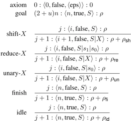
The parser consists of five actions:

axiom 0 :h0,false,hepsii: 0

goal (2 +u)n:hn,true, Si:ρ

shift-X j :hi,false, Si:ρ

j+ 1 :hi+ 1,false, S|Xi:ρ+ρsh

reduce-X j:hi,false, S|s1|s0i:ρ j+ 1 :hi,false, S|Xi:ρ+ρre

unary-X j:hi,false, S|s0i:ρ j+ 1 :hi,false, S|Xi:ρ+ρun

finish j:hn,false, Si:ρ

j+ 1 :hn,true, Si:ρ+ρfi

idle j:hn,true, Si:ρ

j+ 1 :hn,true, Si:ρ+ρid

Figure 1: Deduction system for shift-reduce pars-ing, wherejis a step size andρis a score.

reduce-X pops the top two itemss0ands1out of

the stack and combines them as a partial tree with the constituent labelX as its root, and withs0 ands1 as right and left antecedents,

respectively (X →s1s0). The newly created

tree is then pushed into the stack.

unary-X is similar to reduce-X; however, it con-sumes only the top most item s0 from the stack and pushes a new tree ofX →s0.

finish indicates the completion of parsing, i.e., reaching theROOT.

idle preserves completion until the goal is reached.

The whole procedure is summarized as a deduc-tion system in Figure 1. We employ beam search which starts from an axiom consisting of a stack with a special symbol hepsi, and ends when we reach a goal item (Zhang and Clark, 2009). A set of agenda B = B0, B1,· · · maintains the k-best states for each stepj atBj, which is first initial-ized by inserting the axiom inB0. Then, at each

stepj = 0,1,· · ·, every state in the agendaBj is extended by applying one of the actions and the new states are inserted into the agendaBj+1 for

the next step, which retains only thek-best states. We limit the maximum number of consecutive unary actions tou(Sagae and Lavie, 2005; Zhang and Clark, 2009) and the maximum number of unary actions in a single derivation tou×n. Thus, the process is repeated until we reach the final step

of(2+u)n, which keeps the completed states. The idle action is inspired by the padding method of Zhu et al. (2013), such that the states in an agenda are comparable in terms of score even if differ-ences exist in the number of unary actions. Un-like Zhu et al. (2013) we do not terminate parsing even if all the states in an agenda are completed (f =true).

The score of a state is computed by summing the scores of all the actions leading to the state. In Figure 1, ρ_sh, ρre, ρun, ρfi andρid are the scores

of shift-X, reduce-X, unary-X, finish and idle ac-tions, respectively, which are computed on the ba-sis of the history of actions.

4 Neural Constituent Parsing

The score of a state is defined formally as the total score of transition actions, or a (partial) derivation

d=d0, d1,· · · leading to the state as follows:

ρ(d) =

|d_X|−1

j=0

ρ(dj|dj−0 1). (1)

Note that the score of each action is dependent on all previous actions. In previous studies, the score is computed by a linear model, i.e., a weighted sum of feature values derived from limited histo-ries, such as those that consider two adjacent con-stituent trees in a stack (Sagae and Lavie, 2005; Zhang and Clark, 2009; Zhu et al., 2013). Our method employs an RNN or Elman network (El-man, 1990) to represent an unlimited stack and queue history.

Formally, we use an m-dimensional vector for each hidden state unless otherwise stated. Here, let

xi ∈ Rm0×1 be anm0-dimensional vector repre-senting the input wordwi and the dimension may not match with the hidden state sizem.qi ∈Rm×1 denotes the hidden state for the input wordwiin a queue. Following the RNN in backward direction (Henderson, 2004), the hidden state for each word

wiis computed right-to-left,qn−1toq0, beginning

from a constantqn:

qi =τ(Hquqi+1+Wquxi+bqu), (2)

where Hqu ∈ Rm×m, Wqu ∈ Rm×m0, bqu ∈ Rm×1 _{and τ(x) is hard-tanh applied}

element-wise2_.

h1

j h0j xi xi+1

qi qi+1 h2

j+1h1j+1h0j+1

current stack

next stack queue

input

Hsh

Qsh

Wsh

(a) shift-Xaction

h3

j h2j h1j h0j

qi qi+1 h2

j+1h1j+1h0j+1

current stack next stack

queue

Wre

Qre

Hre

(b) reduce-Xaction

h2

j h1j h0j

qi qi+1 h2

j+1h1j+1h0j+1

current stack next stack

queue

Wun

Hun

Qun

(c) unary-Xaction

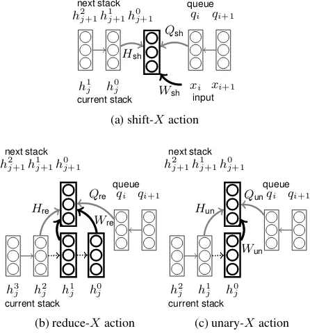
Figure 2: Example neural network for constituent parsing. The thick arrows indicate the context of tree structures, and the gray arrows represent in-teractions from the stack and queue. The dotted arrows denote popped states.

Shift: Now, let hl

j ∈ Rm×1 represent a hidden state associated with thelth stack item for thejth action. We define the score of a shift action:

h0

j+1=τ HshXh0j +QshXqi+WshXxi+bXsh

(3)

ρ(dj =shift-X|dj−₀ 1) =VshXh0j+1+vshX (4)

where HX

sh ∈ Rm×m, QXsh ∈ Rm×m, WshX ∈ Rm×m0

andbX

sh ∈ Rm×1. Figure 2(a) shows the

network structure for Equation 3. HX

shrepresents

an RNN-style architecture that propagates the pre-vious context in the stack. QX

sh can reflect the

queue contextqi, or the future input sequence from

wi through wn−1, while W_shX directly expresses

the leaf of a tree structure using the shifted input word representation xi for wi. The hidden state

h0

j+1 is used to compute the score of a derivation ρ(dj|dj−₀ 1) in Equation 4, which is based on the matrixVX

sh ∈ R1×m and the bias termvshX ∈ R.

Note thathl

j+1 = hl−j 1 for l = 1,2,· · · because the stack is updated by the newly created partial tree labelX associated with the new hidden state

h0

j+1.

Inspired by CVG (Socher et al., 2013), we dif-ferentiate the matrices for each non-terminal (or POS) labelXrather than using shared parameters.

However, our model differs in that the parameters are untied on the basis of the left hand side of a rule, rather than the right hand side, because our model assigns a score discriminatively for each ac-tion with the left hand side labelXunlike a gen-erative model derived from PCFGs.

Reduce: Similarly, the score for a reduce action is obtained as follows:

h0

j+1 =τ

HX

reh2j +QXreqi+WreXh[0:1]j +bXre

(5)

ρ(dj =reduce-X|dj−0 1) =VreXh0j+1+vreX, (6)

where HX

re ∈ Rm×m, QXre ∈ Rm×m, WreX ∈ Rm×2m_,bX

re ∈Rm×1, andh[l:l0]denotes the

verti-cal matrix concatenation of hidden states fromhl tohl0

.

Note that the reduce-X action pops top two items in the stack that correspond to the two hid-den states ofh[0:1]_j as represented by Figure 2(b). By pushing a newly created tree with the con-stituentX, its corresponding hidden stateh0

j+1is

pushed to the stack with each remaining hidden state hl

j+1 = hlj+1 for l = 1,2,· · ·. The hid-den state of the top stack item h0

j is a represen-tation of the right antecedent of a newly created binary tree withh0

j+1 as a root, while the hidden

state of the next top stack item h1

j corresponds to the left antecedent of the binary tree. Thus, the two hidden states capture the recursive neural network-like structure (Costa et al., 2003), while

h2

j =h1j+1represents the RNN-like linear history

in the stack.

Unary: In the same manner as the reduce action, the unary action is defined by simply reducing a single item from a stack and by pushing a new item (Figure 2(c)):

h0_j+1 =τ H_unXh1_j+Q_unXqi+WunXh0j +bXun

(7)

ρ(dj =unary-X|dj−₀ 1) =VunXh0j+1+vunX, (8)

where HX

un ∈ Rm×m, QXun ∈ Rm×m, WunX ∈ Rm×m _andbX

un ∈ Rm×1. Note that hlj+1 = hlj forl = 1,2,· · ·, because only the top item is up-dated in the stack by creating a partial tree withh0

j together with the stack historyh1

j.

finish action and an idle action are defined analo-gous to the unary-Xaction with special labels for

X,hfinishiandhidlei, respectively3_.

5 Parameter Estimation Let θ = HX

sh, QXsh,· · · ∈ RM be an M

-dimensional vector of all model parameters. The parameters are initialized randomly by following Glorot and Bengio (2010), in which the random value range is determined by the size of the in-put/output layers. The bias parameters are initial-ized to zeros.

We employ a variant of max-violation (Huang et al., 2012) as our training objective, in which pa-rameters are updated based on the worst mistake found during search, rather than the first mistake as performed in the early update perceptron al-gorithm (Collins and Roark, 2004). Specifically, given a training instance(w,y)wherewis an in-put sentence andyis its gold derivation, i.e., a se-quence of actions representing the gold parse tree forw, we seek for the stepj∗_{where the difference} of the scores is the largest:

j∗_{= arg min} j

ρθ(yj₀)−max d∈B_jρθ(d)

. (9)

Then, we define the following hinge-loss function:

L(w,y;B,θ) = maxn0,1−ρθ(yj

∗

0 ) +EB˜j∗[ρθ]

o

,

(10)

wherein we consider the subset of sub-derivations

˜

Bj∗ ⊂B_j∗consisting of those scored higher than ρθ(yj

∗ 0 ):

˜ Bj∗ =

n

d∈Bj∗ρ_θ(d)> ρ_θ(y₀j∗)

o

(11)

pθ(d) = P exp(ρθ(d)) d0∈B˜_j∗exp(ρθ(d0))

(12)

E_B˜_j∗[ρθ] =

X

d∈B˜_j∗

pθ(d)ρθ(d). (13)

Unlike Huang et al. (2012) and inspired by Tamura et al. (2014), we consider all incorrect sub-derivations found in B˜j∗ through the expected

score E_B˜_j∗[ρθ]4. The loss function in Equation

3_Sinceh1

jandqnare constants for the finish and idle

ac-tions, we enforceHX

un = 0andQXun = 0for those special

actions.

4_{We can use all the sub-derivations inB}

j∗; however, our

preliminary studies indicated that the use ofB˜j∗was better.

10 can be intuitively considered an expected mis-take suffered at the maximum violated step j∗_, which is measured by the Viterbi violation in Equation 9. Note that if we replaceE_B˜_j∗[ρθ]with maxd∈Bj∗ρθ(d) in Equation 10, it is exactly the same as the max-violation objective (Huang et al., 2012)5_.

To minimize the loss function, we use a di-agonal version of AdaDec (Senior et al., 2013) — a variant of diagonal AdaGrad (Duchi et al., 2011) — under mini-batch settings. Given the sub-gradient g_t ∈ RM _{of Equation 10 at timet} computed by the back-propagation through struc-ture (Goller and K¨uchler, 1996), we maintain ad-ditional parametersGt∈RM:

Gt←γGt−1+gtgt, (14) whereis the Hadamard product (or the element-wise product). θt−1 is updated using the element

specific learning rateη_t ∈ RM _{derived fromGt} and a constantη0>0:

η_t←η0(Gt+)−12 (15)

θ_t−1

2 ←θt−1−ηtgt (16)

θt←arg min θ

1

2kθ−θt−1 2k

2

2+λη>t abs(θ). (17) Compared with AdaGrad, the squared sum of the sub-gradients decays over time using a constant

0 < γ ≤ 1 in Equation 14. The learning rate in Equation 15 is computed element-wise and bounded by a constant≥0, and if we set≥η2

0,

it is always decayed6_{. In our preliminary}

stud-ies, AdaGrad eventually becomes very conserva-tive to update parameters when training longer it-erations. AdaDec fixes the problem by ignoring older histories of sub-gradients inG, which is re-flected in the learning rateη. In each update, we employ`1 regularization through FOBOS (Duchi

and Singer, 2009) using a hyperparameterλ ≥ 0

to control the fitness in Equation 16 and 17. For testing, we found that taking the average of the pa-rameters over period 1

T+1

P_T

t=0θtunder training iterationsTwas very effective as demonstrated by Hashimoto et al. (2013).

Parameter estimation is performed in parallel by distributing training instances asynchronously

5_{Or, settingp}

θ(d∗) = 1for the Viterbi derivationd∗ =

arg maxd∈Bj∗ρθ(d)and zero otherwise.

6_{Note that AdaGrad is a special case of AdaDec withγ=}

in each shard and by updating locally copied pa-rameters using the sub-gradients computed from the distributed mini-batches (Dean et al., 2012). The sub-gradients are broadcast asynchronously to other shards to reflect the updates in one shard. Unlike Dean et al. (2012), we do not keep a cen-tral storage for model parameters; the replicated parameters are synchronized in each iteration by choosing the model parameters from one of the shards with respect to the minimum of`1 norm7.

Note that we synchronizeθ, butGis maintained as shard local parameters.

6 Experiments 6.1 Settings

We conducted experiments for transition-based neural constituent parsing (TNCP) for two lan-guages — English and Chinese. English data were derived from the Wall Street Journal (WSJ) of the Penn Treebank (Marcus et al., 1993), from which sections 2-21 were used for training, 22 for de-velopment and 23 for testing. Chinese data were extracted from the Penn Chinese Treebank (CTB) (Xue et al., 2005); articles 001-270 and 440-1151 were used for training, 301-325 for develop-ment, and 271-300 for testing. Inspired by jack-knifing (Collins and Koo, 2005), we reassigned POS tags for training data using the Stanford tag-ger (Toutanova et al., 2003)8_{. The treebank trees}

were normalized by removing empty nodes and unary rules with X over X (or X → X), then binarized in a left-branched manner.

The possible actions taken for our shift-reduce parsing, e.g., X → w in shift-X, were learned from the normalized treebank trees. The words that occurred twice or less were handled differ-ently in order to consider OOVs for testing: They were simply mapped to a special tokenhunkiwhen looking up their corresponding word representa-tion vector. Similarly, when assigning possible POS tags in shift actions, they fell back to their corresponding “word signature” in the same man-ner as the Berkeley parser9_{. A maximum number}

of consecutive unary actions was set tou = 3for WSJ and u = 4 for CTB, as determined by the 7_{We also tried averaging among shards. However we} ob-served no gains likely because we performed averaging for testing.

8_{http://nlp.stanford.edu/software/} tagger.shtml

9_{https://code.google.com/p/} berkeleyparser/

rep. size 32 64 128 256 512 1024

de

v WSJ-3264 89.91 90.15 90.48 90.70 90.7590.37 90.73 90.81 90.62 90.71 90.8791.11

CTB-32 79.25 81.59 82.80 82.68 84.17 85.12

64 84.04 83.29 82.92 85.12 85.24 85.77

test

WSJ-32 89.03 89.49 89.75 90.45 90.37 90.01 64 89.74 90.16 90.48 90.06 89.91 90.68

CTB-32 75.19 78.29 80.46 81.87 83.16 82.64 64 80.11 81.35 81.67 82.91 83.76 84.33

Table 1: Comparison of various state/word rep-resentation dimension size measured by labeled F1(%). “-32” denotes the hidden state sizem = 32. The numbers in bold indicate the best results for each hidden state dimension.

treebanks.

Parameter estimation was performed on 16 cores of a Xeon E5-2680 2.7GHz CPU. It took approximately one day for 100 training iterations with m = 32 and m0 _{= 128 under a} mini-batch size of 4 and a beam size of 32. Dou-bling either one of m or m0 _incurred approxi-mately double training time. We chose the fol-lowing hyperparameters by tuning toward the de-velopment data in our preliminary experiments10_: η0 = 10−2,γ = 0.9,= 1. The choice ofλfrom {10−5_,10−6_,10−7_{}and the number of training}

it-erations were very important for different training objectives and models in order to avoid overfitting. Thus, they were determined by the performance on the development data for each different train-ing objective and/or network configuration, e.g., the dimension for a hidden state. The word rep-resentations were initialized by a tool developed in-house for an RNN language model (Mikolov et al., 2010) trained by noise contrastive estimation (Mnih and Teh, 2012). Note that the word repre-sentations for initialization were learned from the given training data, not from additional unanno-tated data as done by Chen and Manning (2014).

Testing was performed using a beam size of64

with a Xeon X5550 2.67GHz CPU. All results were measured by the labeled bracketing metric PARSEVAL (Black et al., 1991) using EVALB11

after debinarization. 6.2 Results

Table 1 shows the impact of dimensions on the parsing performance. We varied the hid-10_{We confirmed that this hyperparameter setting was} ap-propriate for different models experimented in Section 6.2 through our preliminary studies.

model tree +stack +queue

de

v WSJ 77.70 90.54 91.11

CTB 69.74 84.70 85.77

test CTBWSJ 76.4866.03 90.0082.85 90.6884.33

Table 2: Comparison of network structures mea-sured by labeled F1(%).

den vector size m = {32,64} and the word representation (embedding) vector size m0 ₌

{32,64,128,256,512,1024}12_{. As can be seen,}

the greater word representation dimensions are generally helpful for both WSJ and CTB on the closed development data (dev), which may match with our intuition that the richer syntactic and se-mantic knowledge representation for each word is required for parsing. However, overfitting was ob-served when using a 32-dimension hidden vector in both tasks, i.e., drops of performance on the open test data (test) when m0 _{= 1024, probably} caused by the limited generalization capability in the smaller hidden state size. In the rest of this pa-per, we show the results withm = 64andm0 ₌

1024 as determined by the performance on the development data, wherein we achieved 91.11% and 85.77% labeled F1 for WSJ and CTB, respec-tively. The total number of parameters were ap-proximately 28.3M and 22.0M for WSJ and CTB, respectively, among which 17.8M and 13.4M were occupied for word representations, respectively.

Table 2 differentiated the network structure. The tree model computes the new hidden state

h0

j+1 using only the recursively constructed

net-work by ignoring parameters from the stack and queue, e.g., by enforcingHX

sh = 0andQXsh = 0

in Equation 3, which is essentially similar to the CVG approach (Socher et al., 2013). Adding the context from the stack in +stack boosts the per-formance significantly. Further gains are observed when the queue context+queueis incorporated in the model. These results clearly indicate that ex-plicit representations of the stack and queue are very important when applying a recursive neural network model for transition-based parsing.

We then compared the expected mistake with the Viterbi mistake (Huang et al., 2012) as our training objective by replacing E_B˜_j∗[ρθ] with

maxd∈B_j∗ρθ(d) in Equation 10. Table 3 shows that the use of the expected mistake (expected) as a loss function is significantly better than that

12_{We experimented larger dimensions in Appendix A.}

loss Viterbi expected

de

v WSJ 90.89 91.11

CTB 84.94 85.77

test CTBWSJ 90.2182.62 90.6884.33

Table 3: Comparison of loss functions measured by labeled F1(%).

65 70 75 80 85 90 95 100

0 10 20 30 40 50 60 70 80 90 100

F1(%)

iterations

expected (train) Viterbi (train) expected (dev) Viterbi (dev)

Figure 3: Plots for training iterations and labeled F1(%) on WSJ.

of the Viterbi mistake (Viterbi) by considering all the incorrect sub-derivations at maximum violated steps during search. Figure 3 and 4 plot the train-ing curves for WSJ and CTB, respectively. The plots clearly demonstrate that the use of the ex-pected mistake is faster in convergence and stabler in learning when compared with that of the Viterbi mistake13_.

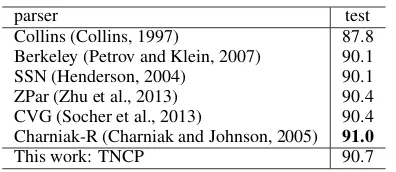
Next, we compare our parser, TNCP, with other parsers listed in Table 4 for WSJ and Table 5 for CTB on the test data. The Collins parser (Collins, 1997) and the Berkeley parser (Petrov and Klein, 2007) are chart-based parsers with rich states, ei-ther through lexicalization or latent annotation. SSN is a left-corner parser (Henderson, 2004), and CVG is a compositional vector grammar-based parser (Socher et al., 2013)14_{. Both parsers rely on}

neural networks to represent rich contexts, similar to our work; however they differ in that they es-sentially perform reranking from either thek-best parses or parse forests15_{. The word}

representa-13_{The labeled F1 on those plots are slightly different from} EVALB in that all the syntactic labels are considered when computing bracket matching. Further, the scores on the train-ing data are approximation since they were obtained as a by-product of online learning.

14_{http://nlp.stanford.edu/software/} lex-parser.shtml

65 70 75 80 85 90 95 100

0 10 20 30 40 50 60 70 80 90 100

F1(%)

iterations

expected (train) Viterbi (train) expected (dev) Viterbi (dev)

Figure 4: Plots for training iterations and labeled F1(%) on CTB.

parser test

Collins (Collins, 1997) 87.8 Berkeley (Petrov and Klein, 2007) 90.1

SSN (Henderson, 2004) 90.1

ZPar (Zhu et al., 2013) 90.4 CVG (Socher et al., 2013) 90.4 Charniak-R (Charniak and Johnson, 2005) 91.0

This work: TNCP 90.7

Table 4: Comparison of different parsers on the WSJ test data measured by labeled F1(%).

tion in CVG was learned from large monolingual data (Turian et al., 2010), but our parser learns word representation from only the provided train-ing data. Charniak-R is a discriminative rerank-ing parser with non-local features (Charniak and Johnson, 2005). ZPar is a transition-based shift-reduce parser (Zhu et al., 2013)16 _{that influences}

the deduction system in Figure 1, but differs in that scores are computed by a large number of features and POS tagging is performed separately. The re-sults shown in Table 4 and 5 come from the feature set without extra data, i.e., semi-supervised fea-tures. Joint is the joint POS tagging and transition-based parsing with non-local features (Wang and Xue, 2014). Similar to ZPar, we present the result without cluster features learned from extra unan-notated data.

Finally, we measured the speed for parsing by varying beam size and hidden dimension (Table 6). When testing, we applied a pre-computation technique for layers involving word representation vectors (Devlin et al., 2014), i.e.,Wquin Equation

2 andWX

shin Equation 3. Thus, the parsing speed

was influenced by only the hidden state sizem. It is clear that the enlarged beam size improves per-16_{http://sourceforge.net/projects/zpar/}

parser test

ZPar (Zhu et al., 2013) 83.2 Berkeley (Petrov and Klein, 2007) 83.3 Joint (Wang and Xue, 2014) 84.9

This work: TNCP 84.3

Table 5: Comparison of different parsers on the CTB test data measured by labeled F1(%).

beam 32 64 128

WSJ-32 15.42/89.95 7.90/90.01 3.97/90.04

64 7.31/90.56 3.56/90.68 1.76/90.73

CTB-32 13.67/82.35 6.95/82.64 3.68/82.84

64 6.15/84.12 3.11/84.33 1.53/83.83

Table 6: Comparison of parsing speed by varying beam size and hidden dimension; each cell shows the number of sentences per second/labeled F1(%) measured on the test data.

formance by trading off run time in most cases. Note that Berkeley, CVG and ZPar took 4.74, 1.54 and 37.92 sentences/sec, respectively, with WSJ. Although it is more difficult to compare with other parsers, our parser implemented in C++ is on par with Java implementations of Berkeley and CVG. The large run time difference with the C++ imple-mented ZPar may come from the network compu-tation and joint POS inference in our model which impact parsing speed significantly.

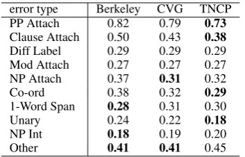
6.3 Error Analysis

To assess parser error types, we used the tool pro-posed by Kummerfeld et al. (2012)17_{. The average}

number of errors per sentence is listed in Table 7 for each error type on the WSJ test data. Gener-ally, our parser results in errors that are compara-ble to the state-of-the-art parsers; however, greater reductions are observed for various attachments errors. One of the largest gains comes from the clause attachment, i.e., 0.12 reduction in average errors from Berkeley and 0.05 from CVG. The av-erage number of errors is also reduced by 0.09 from Berkeley and 0.06 from CVG for the PP at-tachment. We also observed large reductions in coordination and unary rule errors.

7 Conclusion

We have introduced transition-based neural con-stituent parsing — a neural network architecture that encodes each state explicitly — as a con-tinuous vector by considering the recurrent

error type Berkeley CVG TNCP PP Attach 0.82 0.79 0.73

Clause Attach 0.50 0.43 0.38

Diff Label 0.29 0.29 0.29 Mod Attach 0.27 0.27 0.27 NP Attach 0.37 0.31 0.32

Co-ord 0.38 0.32 0.29

1-Word Span 0.28 0.31 0.30

Unary 0.24 0.22 0.18

NP Int 0.18 0.19 0.20

Other 0.41 0.41 0.45

Table 7: Comparison of different parsers on the WSJ test data measured by average number of er-rors per sentence; the numbers in bold indicate the least errors in each error type.

quences of the stack and queue in the transition-based parsing framework in addition to recursively constructed partial trees. Our parser works in a standalone fashion without reranking and does not rely on an external POS tagger or additional monolingual data for reliable estimates of syntac-tic and/or semansyntac-tic representations of words. The parser achieves performance that is comparable to state-of-the-art systems.

In the future, we plan to apply our neural net-work structure to dependency parsing. We are also interested in using long short-term memory neu-ral networks (Hochreiter and Schmidhuber, 1997) to better model the locality of propagated infor-mation from the stack and queue. The parameter estimation under semi-supervised setting will be investigated further.

Acknowledgments

We would like to thank Lemao Liu for suggestions while drafting this paper. We are also grateful for various comments from anonymous reviewers.

References

George Berg. 1992. A connectionist parser with recur-sive sentence structure and lexical disambiguation. InProc. of AAAI ’92, pages 32–37.

Ezra Black, Steve Abney, Dan Flickinger, Claudia Gdaniec, Ralph Grishman, Phil Harrison, Don Hin-dle, Robert Ingria, Fred Jelinek, Judith Klavans, Mark Liberman, Mitchell Marcus, Salim Roukos, Beatrice Santorini, and Tomek Strzalkowski. 1991. Procedure for quantitatively comparing the

syntac-tic coverage of english grammars. InProc. of the

Workshop on Speech and Natural Language, pages 306–311, Stroudsburg, PA, USA.

Eugene Charniak and Mark Johnson. 2005. Coarse-to-fine n-best parsing and maxent discriminative

reranking. In Proc. of ACL 2005, pages 173–180,

Ann Arbor, Michigan, June.

Eugene Charniak. 2000. A

maximum-entropy-inspired parser. In Proc. of NAACL 2000, pages

132–139, Stroudsburg, PA, USA.

Danqi Chen and Christopher Manning. 2014. A fast and accurate dependency parser using neural

net-works. InProc. of EMNLP 2014, pages 740–750,

Doha, Qatar, October.

Michael Collins and Terry Koo. 2005. Discriminative

reranking for natural language parsing.

Computa-tional Linguistics, 31(1):25–70, March.

Michael Collins and Brian Roark. 2004. Incremental

parsing with the perceptron algorithm. InProc. of

ACL 2004, pages 111–118, Barcelona, Spain, July. Michael Collins. 1997. Three generative, lexicalised

models for statistical parsing. InProc. of ACL ’97, pages 16–23, Madrid, Spain, July.

Michael Collins. 2003. Head-driven statistical models

for natural language parsing. Computational

Lin-guistics, 29(4):589–637, December.

Fabrizio Costa, Paolo Frasconi, Vincenzo Lombardo, and Giovanni Soda. 2003. Towards incremental parsing of natural language using recursive neural networks. Applied Intelligence, 19(1-2):9–25, May. Jeffrey Dean, Greg Corrado, Rajat Monga, Kai Chen, Matthieu Devin, Mark Mao, Marc’aurelio Ranzato, Andrew Senior, Paul Tucker, Ke Yang, Quoc V. Le, and Andrew Y. Ng. 2012. Large scale distributed

deep networks. InAdvances in Neural Information

Processing Systems 25, pages 1223–1231. Curran Associates, Inc.

Jacob Devlin, Rabih Zbib, Zhongqiang Huang, Thomas Lamar, Richard Schwartz, and John Makhoul. 2014. Fast and robust neural network joint models for sta-tistical machine translation. InProc. of ACL 2014, pages 1370–1380, Baltimore, Maryland, June. John Duchi and Yoram Singer. 2009. Efficient online

and batch learning using forward backward splitting.

Journal of Machine Learning Research, 10:2899– 2934, December.

John Duchi, Elad Hazan, and Yoram Singer. 2011. Adaptive subgradient methods for online learning

and stochastic optimization. Journal of Machine

Learning Research, 12:2121–2159, July.

Jeffrey L. Elman. 1990. Finding structure in time.

Cognitive Science, 14(2):179–211.

Xavier Glorot and Yoshua Bengio. 2010. Understand-ing the difficulty of trainUnderstand-ing deep feedforward neural

networks. In Proc. of the Thirteenth International

Christoph Goller and Andreas K¨uchler. 1996. Learn-ing task-dependent distributed representations by

backpropagation through structure. In Proc. of

IEEE International Conference on Neural Networks, 1996, volume 1, pages 347–352 vol.1, Jun.

David Hall, Greg Durrett, and Dan Klein. 2014. Less

grammar, more features. In Proc. of ACL 2014,

pages 228–237, Baltimore, Maryland, June.

Kazuma Hashimoto, Makoto Miwa, Yoshimasa Tsu-ruoka, and Takashi Chikayama. 2013. Simple cus-tomization of recursive neural networks for seman-tic relation classification. InProc. of EMNLP 2013, pages 1372–1376, Seattle, Washington, USA, Octo-ber.

James Henderson. 2003. Inducing history represen-tations for broad coverage statistical parsing. In

Proc. of HLT-NAACL 2003, pages 24–31, Strouds-burg, PA, USA.

James Henderson. 2004. Discriminative training of a

neural network statistical parser. In Proc. of ACL

2004, pages 95–102, Barcelona, Spain, July.

Sepp Hochreiter and J¨urgen Schmidhuber. 1997.

Long short-term memory. Neural Computation,

9(8):1735–1780, November.

Liang Huang, Suphan Fayong, and Yang Guo. 2012. Structured perceptron with inexact search. InProc. of NAACL-HLT 2012, pages 142–151, Montr´eal, Canada, June.

Dan Klein and Christopher D. Manning. 2003. Ac-curate unlexicalized parsing. InProc. of ACL 2003, pages 423–430, Sapporo, Japan, July.

Jonathan K. Kummerfeld, David Hall, James R. Cur-ran, and Dan Klein. 2012. Parser showdown at the wall street corral: An empirical investigation of error

types in parser output. InProc. of EMNLP-CoNLL

2012, pages 1048–1059, Jeju Island, Korea, July.

Phong Le and Willem Zuidema. 2014. The inside-outside recursive neural network model for

depen-dency parsing. In Proc. of EMNLP 2014, pages

729–739, Doha, Qatar, October.

Mitchell P. Marcus, Mary Ann Marcinkiewicz, and Beatrice Santorini. 1993. Building a large

anno-tated corpus of english: The penn treebank.

Compu-tational Linguistics, 19(2):313–330, June.

Takuya Matsuzaki, Yusuke Miyao, and Jun’ichi Tsujii. 2005. Probabilistic CFG with latent annotations. In

Proc. of ACL 2005, pages 75–82, Ann Arbor, Michi-gan, June.

Marshall R. Mayberry and Risto Miikkulainen. 1999. Sardsrn: A neural network shift-reduce parser. In

Proc. of IJCAI ’99, pages 820–827, San Francisco, CA, USA.

Sauro Menchetti, Fabrizio Costa, Paolo Frasconi, and Massimiliano Pontil. 2005. Wide coverage natural language processing using kernel methods and

neu-ral networks for structured data. Pattern

Recogni-tion Letters, 26(12):1896–1906, September.

Tom´aˇs Mikolov, Martin Karafi´at, Luk´aˇs Burget, Jan ˇCernock´y, and Sanjeev Khudanpur. 2010.

Recur-rent neural network based language model. InProc.

of INTERSPEECH 2010, pages 1045–1048.

Andriy Mnih and Yee W. Teh. 2012. A fast and simple algorithm for training neural probabilistic language models. In John Langford and Joelle Pineau,

edi-tors, Proc. of ICML-2012, pages 1751–1758, New

York, NY, USA.

Slav Petrov and Dan Klein. 2007. Improved inference

for unlexicalized parsing. InProc. of NAACL-HLT

2007, pages 404–411, Rochester, New York, April.

Slav Petrov, Leon Barrett, Romain Thibaux, and Dan Klein. 2006. Learning accurate, compact, and

inter-pretable tree annotation. InProc. of COLING-ACL

2006, pages 433–440, Sydney, Australia, July.

Jordan B. Pollack. 1990. Recursive distributed repre-sentations. Artificial Intelligence, 46(1-2):77–105, November.

Kenji Sagae and Alon Lavie. 2005. A classifier-based parser with linear run-time complexity. In

Proc. of the Ninth International Workshop on Pars-ing Technology, pages 125–132, Vancouver, British Columbia, October.

Andrew Senior, Georg Heigold, Marc’Aurelio Ran-zato, and Ke Yang. 2013. An empirical study of learning rates in deep neural networks for speech

recognition. InProc. of ICASSP 2013, pages 6724–

6728, May.

Richard Socher, John Bauer, Christopher D. Manning, and Ng Andrew Y. 2013. Parsing with

compo-sitional vector grammars. In Proc. of ACL 2013,

pages 455–465, Sofia, Bulgaria, August.

Pontus Stenetorp. 2013. Transition-based dependency

parsing using recursive neural networks. In Proc.

of Deep Learning Workshop at the 2013 Conference on Neural Information Processing Systems (NIPS), Lake Tahoe, Nevada, USA, December.

Akihiro Tamura, Taro Watanabe, and Eiichiro Sumita. 2014. Recurrent neural networks for word

align-ment model. In Proc. of ACL 2014, pages 1470–

1480, Baltimore, Maryland, June.

Kristina Toutanova, Dan Klein, Christopher D. Man-ning, and Yoram Singer. 2003. Feature-rich part-of-speech tagging with a cyclic dependency

net-work. In Proc. of HLT-NAACL 2003, pages 173–

rep. size 32 64 128 256 512 1024 2048 4096

de

v WSJ-3264 89.91 90.15 90.48 90.70 90.75 90.8790.37 90.73 90.81 90.62 90.71 91.11 91.3491.11 91.0491.36

CTB-32 79.25 81.59 82.80 82.68 84.17 85.12 85.61 85.76

64 84.04 83.29 82.92 85.12 85.24 85.77 86.28 86.94

test

WSJ-32 89.03 89.49 89.75 90.45 90.37 90.01 90.33 90.40 64 89.74 90.16 90.48 90.06 89.91 90.68 91.05 90.94 CTB-32 75.19 78.29 80.46 81.87 83.16 82.64 83.13 83.67

64 80.11 81.35 81.67 82.91 83.76 84.33 83.76 84.38

Table 8: Comparison of various state/word representation dimension size measured by labeled F1(%). “-32” denotes the hidden state sizem= 32. The numbers in bold indicate the best results for each hidden state dimension.

Joseph Turian, Lev-Arie Ratinov, and Yoshua Bengio. 2010. Word representations: A simple and general

method for semi-supervised learning. In Proc. of

ACL 2010, pages 384–394, Uppsala, Sweden, July. Zhiguo Wang and Nianwen Xue. 2014. Joint pos

tag-ging and transition-based constituent parsing in chi-nese with non-local features. InProc. of ACL 2014, pages 733–742, Baltimore, Maryland, June.

Naiwen Xue, Fei Xia, Fu-dong Chiou, and Marta Palmer. 2005. The penn chinese treebank: Phrase structure annotation of a large corpus. Natural Lan-guage Engineering, 11(2):207–238, June.

Yue Zhang and Stephen Clark. 2009. Transition-based parsing of the chinese treebank using a global dis-criminative model. InProc. of the 11th International Conference on Parsing Technologies (IWPT’09), pages 162–171, Paris, France, October.

Muhua Zhu, Yue Zhang, Wenliang Chen, Min Zhang, and Jingbo Zhu. 2013. Fast and accurate

shift-reduce constituent parsing. In Proc. of ACL 2013,

pages 434–443, Sofia, Bulgaria, August.

A Additional Results