Munich Personal RePEc Archive
Comparative Determinants of Quality of
Growth in Developing Countries
Asongu, Simplice and Asongu, Ndemaze
January 2017
Online at
https://mpra.ub.uni-muenchen.de/80650/
1
A G D I Working Paper
WP/17/013
Comparative Determinants of Quality of Growth in Developing Countries
Forthcoming in: International Journal of Happiness and Development
Simplice A. Asongu
African Governance and Development Institute, P.O. Box 8413 Yaoundé, Cameroon. E-mail: [email protected]
Ndemaze Asongu
African Governance and Development Institute, P.O. Box 8413 Yaoundé, Cameroon. E-mail: [email protected]
Department of Communication Sciences Faculty of Humanities
2
2017 African Governance and Development Institute WP/17/013
Research Department
Comparative Determinants of Quality of Growth in Developing Countries
Simplice A. Asongu & Ndemaze Asongu
January 2017
Abstract
This study explores a new dataset in order to present the comparative determinants of growth
quality in 93 developing countries for the period 1990-2011. We employ both cross-sectional
and panel estimation techniques with contemporary and non-contemporary specifications. The
determinants are quite heterogeneous in significance and magnitude with substantial
inclinations to specifications and estimation techniques. We present and discuss the findings
in increasing magnitude of significance so as to ease comparative readability. We also discuss
how specificities in the modelling techniques are relevant for targeting growth quality. The
results are timely and relevant for the post-2015 inclusive and sustainable development
agenda.
JEL Classification: O40; O57; I10; I20; I32
3
1. Introduction
The study on determinants of the quality of growth index (QGI) documented by Mlachila et
al. (2014) leave room for improvement in three areas: (i) data, (ii) methodology and (iii) need
to report and interpret estimated coefficients (Asongu & Nwachukwu, 2017a)1. First, the
relevance of improving data is threefold. (i) We provide determinants based on 17
fundamental characteristics (or sub-panels) of development as opposed to the 7 documented
by the underlying study (p. 30)2. In addition to those clearly articulated but unexploited by
the underlying paper3, we also derive three sub-panels based on time-consistent ‘quality of
growth’ performance that are not explicitly circumvented (p. 16). These include: Best
Performers, Hopefuls and Contenders in growth quality4. The interest of doing so is to
provide more options to policy makers. (ii) The dimension of social spending used in the
paper is decomposed into its educational and health components to provide more room for
policy implications. (iii) The underlying study introduces the ‘rule of law’, ‘corruption
-control’ and ‘aggregate institutional quality’ into the same specifications. This results in
issues of multicollinearity owing to high degrees of substitutions among the variables. We
avoid this specification issue in order to prevent estimated coefficients (with a high degree of
substitution) emerging with unexpected signs.
1
The QGI is composed of two main components, notably: (i) growth fundamentals (strength, volatility, sectoral composition and demand composition) and (ii) social outcomes (health and education). Hence, the proposed QGI entails both social dimensions and the intrinsic nature of economic growth. Accordingly, the QGI goes beyond the well established Human Development Index (HDI) developed by the United Nations by not exclusively concentrating on the levels of incomes, but also on the very nature of growth.
2
The 17 fundamental characteristics are sub panels by which the dataset is disaggregated. This include Growth Quality (GQ) performance (Hopefuls (Hope), Contenders (Cont) and Best performers (Best)); State fragility (Fragile (Frag) and Non-Fragile (Non-Fragile) countries); resource-wealth (Resource-rich (RR), Resource-poor (RP)); income levels (Low-income (LIC), Middle-income (MIC), Lower-middle-income (LMIC) and Upper-middle-income (UMIC); regions (Sub-Saharan Africa (SSA), Middle East & North Africa (MENA), Asia & Pacific (AP), Central & Eastern Europe (CEE) and Latin America(LA)) and non-overlapping intervals (1990-1994; 1995-1999; 2000-2004 & 2005-2011).
3
Fundamental sub-panels are depicted in Figures 2-3 (pp. 13-14) and Figure 4 (p. 16). We employ ‘underlying
study’ and Mlachila et al. (2014) interchangeably.
4
4 Second, on the methodological front, the regressions employed are one lagged
non-contemporary Ordinary Least Squares (OLS) estimations for the Full sample (p. 21) and
contemporary estimations for 7 sub-samples (p. 30). We improve this dimension in three main
areas: data structure, time-oriented specifications and a complementarity of OLS. (1) Both
cross-sectional and panel specifications are employed in the current study. The former is
time-dynamic to enable an appreciation across time. (2) The specifications are both contemporary
and non-contemporary to offer more insights into the linkages. (3) OLS are complemented
with Fixed Effects (FE) or Random-Effects (RE) regressions depending on the outcome of the
Hausman test for endogeneity. The adopted FE regressions control for the unobserved
heterogeneity.
Third, we do not limit the reporting and interpretation of estimated coefficients to their
signs (p. 30). Hence, we also discuss their magnitudes across specifications and fundamental
characteristics. Building on the above, this study investigates the determinants of quality of
growth in developing countries with particular emphasis on fundamental characteristics of
inclusive growth.
The policy relevance of the study builds the fact that the conception, definition and
measurement of ‘inclusive growth’ employed as the outcome indicator in this study is in line
with at least six of the seventeen Sustainable Development Goals (SDGs), namely: Goal
1(‘end poverty in all its forms everywhere’), Goal 2 (‘end hunger, achieve food security and
improved nutrition and promote sustainable agriculture’); Goal 3 (‘ensure healthy lives and
promote well-being for all ages’); Goal 4 (‘ensure inclusive and equitable quality education
and promote lifelong learning opportunities for all’); Goal 8 (‘promote sustained, inclusive
and sustainable economic growth, full and productive employment and decent work for all’ )
5 The remainder of the paper is organized in the following manner. Contemporary issues
on growth and inclusive development are covered in Section 2. Section 3 discusses the data
and methodology. The empirical analysis and discussion of results are covered in Section 4.
Section 5 presents concluding implications.
2. Contemporary issues in growth and inclusive development
The transition from Millennium Development Goals (MDGs) to SDGs after 2015 calls for
inclusive growth strategies because sustained growth is sustainable when it is inclusive: “In
fact, sustained growth plus inclusive growth is sustainable growth, which is the objective
dimension of sustainable development” (Asongu et al., 2014, p.11). This narrative is
consistent with the substantially documented critical dimension of income-inequality in
growth-poverty relationships (Thorbecke, 2013). In essence, because the growth elasticity of
poverty is lower than the inequality elasticity of poverty, the poverty-growth nexus is a
decreasing function of inequality (Fosu, 2015; Asongu & Nwachukwu, 2016a). The assertion
has been consistently verified and confirmed in developing countries5.
The association of output with negative income externalities or “immiserizing growth”
reminds scholars of Lewis: “Output may be growing, and yet the mass of the people may be
becoming poorer” (Lewis, 1955). “Lewis led all developing countries to water, proverbially
speaking, some African countries have so far chosen not to drink” (Amavilah, 2014, p. 2). In
essence, the recent evidence of Africa ‘being on time’ for some MDGs extreme poverty
targets (Pinkivskiy & Sala-i-Martin, 2014) is also being contrasted with stylized facts
5
The conclusions are valid for African (Fosu, 2008, 2009, 2010a, 2010b) as well as a broader sample of
developing nations (Fosu, 2010c). The interested reader can refer to, inter alia: “The study finds that the
6 documenting that inequality is limiting the equal distribution of fruits from economic
prosperity (Blas, 2014)6.
Recent inclusive growth literature has focused on, inter alia: gender inequality
(Anyanwu, 2014a, 2013a; Baliamoune-Lutz, 2007; Baliamoune-Lutz, 2007 & McGillivray,
2009; Elu & Loubert, 2013), relationships between finance, growth, employment and poverty
(Odhiambo, 2009, 2011), the role of finance in poverty eradication (Odhiambo, 2010a,
2010b, 2013; Asongu & Nwachukwu, 2017b, 2017c), linkages between mobile banking,
human development and information technology in inclusive development (Asongu &
Nwachukwu, 2017c; Asongu & Le Roux, 2017), correlates of poverty (Anyanwu, 2014b,
2013b), debates over absolute pro-poor (Ravallion & Chen, 2003) versus relative pro-poor
growth (Dollar & Kraay, 2002) and measurements and determinants of inclusive growth
(Anand et al., 2013; Mlachila et al., 2014). The last strand is closest to the present inquiry
which assesses determinants of inclusive growth in developing countries.
An inclusive growth indicator that accounts for inequality has been proposed by
Anand et al. (2013). It is motivated by an underlying literature on the need for inclusive
growth to encompass growth that reduces poverty sustainably (Kraay, 2004; Berg et al.,
2011ab). The adopted concept of growth in the measurement is absolute pro-poor growth,
maintains that for growth to be inclusive it must benefit the poor absolutely (Ravallion &
Chen, 2003). The authors have argued that the alternative version or relative pro-poor growth
which maintains that growth is inclusive only when it mitigates inequality through positive
income benefits for the poor (see Dollar & Kraay, 2002), could be associated with
sub-optimal externalities for majority of poor and rich households. Moreover, the definition of
inclusiveness and conception of inclusive growth encapsulate characteristics, like: equal
6
It is also important to note that, narratives of the African growth miracle are contingent on the periodicity of
study (Young, 2012). Therefore, compared to the 1980-2010 period, the continent’s relative better poverty
7 opportunities, equity, employment transitions and market protection. Hence, the inclusive
growth measurement entails increasing growth and economic expansion via level-playing
fields of employment, evolving investment and productivity (Anand et al., 2013).
Mlachila et al. (2014) have complemented Anand et al. (2013) by combining previous
concepts, definitions and appreciations of pro-poor growth into a new indicator, termed
‘quality of growth’. The index also builds on an evolving literature on inclusive growth (see
Ianchovichina & Gable, 2012; Commission on Growth & Development, 2008). Building on
the evidence that growth in sub-Saharan Africa has not been associated with reduction in
inequality, poverty and unemployment (Dollar & Kraay, 2002; Martinez & Mlachila, 2013;
Dollar et al., 2013; Ola-David & Oyelaran-Oyeyinka, 2014), the indicator considers inclusive
growth as pro-poor growth that is high, durable and socially friendly. Therefore, according to
the narrative, certain features are essential for growth quality, among others: strength,
stability, growing productivity, sustainability and socially-friendly outcomes like better living
standards and poverty reduction. The present inquiry extends Mlachila et al. (2014) because it
has incorporated social dimensions into the intrinsic value of growth.
The positioning of the inquiry complements the literature which has criticised
Piketty’s literature by emphasising the need to include developing countries in the debate.
Piketty’s celebrated ‘capital in the 21st century’ (Piketty, 2014) has substantially debunked the
Kuznets’ (1955, 1971) orthodoxy on an inverted U-shaped nexus between inequality and
industrialization, paving the way to many evolving strands in the literature. (i) The causes of
inequality, inter alia: globalization-driven debts, theorized by Azzimonti et al. (2014) in
OECD7 nations and partially confirmed in African countries (Asongu et al., 2015) and
adulterated democracy (Stiglitz, 2014). (ii) The consequences of inequality, like increasing
poverty and diminishing growth (Ncube et al., 2014). (iii) Commentary-based responses such
7
8 as cross-checking of facts (Branko, 2014; Krusell & Smith, 2014), reviews (Allen, 2014;
Homburg, 2014) and data quality analysis (Reynolds, 2014). (iv) The neglect of developing
countries where the poor by Piketty’s standard is super-rich in some developing countries
(Asongu & Nwachukwu, 2016b).
3. Data and Methodology
3.1 Data and fundamental characteristics
We investigate a sample of 93 developing nations with data from Mlachila et al.
(2014) for the period 1990-2011. The publicly available dataset is in non-overlapping
averages: 1990-1994; 1995-1999; 2000-2004 and 2005-2011. The authors have computed the
quality of growth index (QGI) using data from various sources, among others: World
Development Indicators of the World Bank, Barro and Lee (2010), Sala-i-Martin (2006), the
International Monetary Fund’s (IMF’s) World Economic Outlook database and the United
Nation’s (UN’s) COMTRADE database.
Two steps are followed in the construction of the QGI, notably: the first set of
variables are standardized to produce indices of symmetric scale and (ii) then aggregated
using different weights to derive a single composite index. It is important to note that the
plethora of indicators used is not expressed in the same units in order to achieve the
aggregated single index. Two main approaches are employed to tackle the concern of
different measurement units, namely: the Min-Max approach and the Z-score or
centered-reduced normalization approach.
The dependent variable is the QGI while determinants which are consistent with the
underlying study include: health spending, education spending, inflation, government
stability, foreign direct investment (FDI), private domestic credit, remittances, quality of
bureaucracy, foreign aid, and rule of law. A complete definition of the variables is presented
9 As discussed in the introduction, two main differences characterize the dataset, relative
to the underlying study. First, we have disaggregated the variable of social spending into its
education and health components. Second, we do not incorporate indicators with a high
degree of substitution8. Hence, we have used the rule of law indicator and dropped
corruption-control and aggregated institutional quality because the three are highly
correlated.
The independent variables used by the underlying study which are in accordance with
Anand et al. (2013, p. 16) are justified by a bulk of inclusive growth literature. With the
exception of inflation which should naturally mitigate growth quality because of decreasing
purchasing power, other determinants should have expected positive signs for the most part.
It should be noted that only high inflation potentially mitigates growth quality. Accordingly,
low/stable inflation may have positive income-equalization effects because it stimulates
private consumption and investment needed to boost economic growth (Asongu, 2013). The
justifications provided for the positive signs are based on a broad stream of inclusive growth
literature (Barro & Lee, 2000; Anand et al., 2012; Mishra, et al., 2011; Calderon & Servén,
2004; Dollar & Kraay, 2003; Seneviratne & Sun, 2013; Levine, 2005; IMF, 2007; Hausmann
et al., 2007).
As maintained by the IMF (2007) and Anand et al. (2013), macroeconomic stability,
structural change and human capital are important pro-poor growth drivers in developing
nations. While the second (or structural change) embodies globalisation (trade openness &
FDI) the first and third entail features that have been documented as growth factors in the
catch-up literature (educational levels, fixed investment and technological change). Other
macroeconomic fundamentals and structural features entail: financial development (Levine,
8
10 2005); inflation and volatility of output (Dollar & Kraay, 2003; Barro & Lee, 2010);
improving status in the value chain ladder of commodities (Hausmann et al., 2007; Anand et
al., 2012); infrastructural quality improvement (Seneviratne & Sun, 2013; Calderon & Servén,
2004) and modernizing production processes (Mishra et al., 2011).
Appendix 2 presents the summary statistics which shows that the variables are
comparable based on some considerable degree of variation. Hence, we can be certain that
some reasonable estimated linkages would emerge. Potential concerns of multicollinearity are
mitigated with the correlation matrix in Appendix 3. Sub-panels are based on five criteria
from which we derive 17 fundamental features9. The multiple characteristics enable us to
extend concerns about heterogeneity in factors presented in Table 3 (p. 21) of the underlying
study. The additional features which are derived from Figures 2-3 (pp. 13-14) and Figure 4 (p.
16) include: GQ performance (Hopefuls (Hope), Contenders (Cont) and Best performers
(Best)); State fragility (Fragile (Frag) and Non-Fragile (Non-Fragile) countries);
resource-wealth (Resource-rich (RR), Resource-poor (RP)); income levels (Low-income (LIC),
Middle-income (MIC), Lower-middle-income (LMIC) and Upper-middle-income (UMIC);
regions (Sub-Saharan Africa (SSA), Middle East & North Africa (MENA), Asia & Pacific
(AP), Central & Eastern Europe (CEE) and Latin America(LA)) and non-overlapping
intervals (1990-1994; 1995-1999; 2000-2004 & 2005-2011).
3.2 Methodology
Contemporary and non-contemporary comparative determinants are assessed from
both cross-sectional and panel specifications. While panel specifications are contemporary
and non-contemporary, cross-sectional regressions are only non-contemporary owing to the
nature of the data structure. In the former specifications, Heteroscedasticity and
Autocorrelation Consistent (HAC) standard errors OLS are used to complement Fixed Effects
9
11 (FE) regressions. A Hausman test is employed to assess the presence of endogeneity prior to
the FE specifications that control for the unobserved heterogeneity. The cross-sectional
contemporary regressions are Heteroscedasticity-consistent.
The following are steps in the estimation process.
Step 1: Cross-sectional contemporary determinants (Table 1)
i i j j j i W
QGI
,
10
1
(1)
This OLS estimation is based on Heteroscedasticity consistent standard errors (SE)
Step 2: Baseline Panel contemporary determinants (Table 2)
t i t i j j j t i W
QGI ,, ,
10
1
,
(2)
Where: QGIi,t is the Quality of Growth Index for country i at period t; is a constant, W is
the vector of determinants and i,t the error term.
Step 3: Baseline Panel non-contemporary determinants (Table 3)
t i t i j j j t i W
QGI ,, 1 , 10
1
,
(3)Eqs (2) and (3) are based on HAC standard errors OLS.
Step 4: Panel Fixed Effects contemporary determinants (Table 4)
t i t i t i j j j t i W
QGI ,, ,
10
1
,
(4)
Where, iis the country-specific effect and tis the time-specific effect.
Step 5: Panel Fixed Effects non-contemporary determinants (Table 5)
t i t i t i j j j t i W
QGI ,, 1 ,
10
1
,
12 Eqs (4) and (5) are based HAC standard errors with control for both country-specific and time
effects. The choice of the Fixed Effects model is justified by a significant Hausman test for
endogeneity.
4. Empirical results
4.1. Cross-sectional determinants
Table 1 below which presents cross-sectional regressions based on Eq. (1), broadly confirms
findings of the underlying study, with the exception of inflation (rule of law) that has a
positive (negative) effect. It provides three clarifications in relation to the underlying paper,
notably: (i) the positive correlation of domestic credit is most apparent in the period
2005-2011; (ii) the positive correlation of FDI is more visible in the periods 1995-1999 and
2000-2004; (iii) the negative correlation of foreign aid is not apparent during the 2005-2011
interval and (iv) the rule of law is negatively linked to growth quality in the initial period
(1990-1994).
“Insert Table 1 here”
4.2 Panel determinants
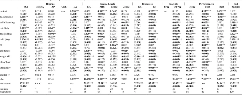
Table 2, Table 3, Table 4 and Table 5 below respectively present ‘baseline contemporary
determinants in HAC SE OLS’10, ‘baseline no
n-contemporary determinants in HAC SE OLS’,
‘HAC SE Panel FE’11 contemporary determinants’ and ‘HAC SE Panel FE’
non-contemporary determinants. Tables 2-5 are also respectively consistent with Eqs. (2)-(5). Our
three-step line of interpretation is simple to follow. For every table and in chronological order,
we discuss: (i) expected and unexpected signs; (ii) the findings in relation to the underling
paper and (iii) comparative evidence between sub-samples in terms of signs and magnitudes.
10
Heteroscedasticity and Autocorrelation Consistent (HAC) Standard Errors (SE) Ordinary Least Squares (OLS).
11
13 The following can be established for Table 2. First, the estimated coefficients in terms
of expected signs are very heterogeneous. Second, the findings are also not broadly consistent
with the underlying paper. Third, we compare the estimates in chronological (or from
education to bureaucracy) and increasing order of magnitude in significance. (i) Education
spending is positively (negatively) significant for LIC, SSA and Contenders (LA & Best
Performers). (ii) Health spending is consistently positive in: LA, RP, UMIC, NFrag, Full
Sample and Contenders. (iii) With the exception of LA, government stability is positive in:
{NFrag, Full Sample}12, Contenders, LIC, SSA, Hopefuls and AP. (iv) The effect of inflation
is consistently positive: MIC, {NFrag, Full Sample}, Hopefuls, {RP, LIC}, SSA and AP. (v)
With the exception of Contenders, the impact of domestic private credit is also
overwhelmingly positive: SSA, {RP, Hopefuls}, LIC, {NFrag, Full Sample}, LIMC, RR and
MENA. (vi) The impacts of FDI are also consistently positive: Full Sample, {LA, LMIC,
NFrag, Contenders}, {Best Performers & MIC}. (vii) On the incidence of remittances, but for
LA, the following are appealing: RP, Contenders, {Hopefuls, LIC} and UMIC. (viii)
Excluding AP, foreign aid has a negative impact in: Hopefuls, {SSA, LIC}, LMIC, {RP,
NFrag, Full Sample}, RR and UMIC. (ix) The rule of law is sparingly negative in: Hopefuls
and Contenders. (x) The impact of bureaucratic quality is consistently positive in: Hopefuls,
SSA, LIC, RR, RP, Full Sample, LA, NFrag and UMIC.
“Insert Table 2 here”
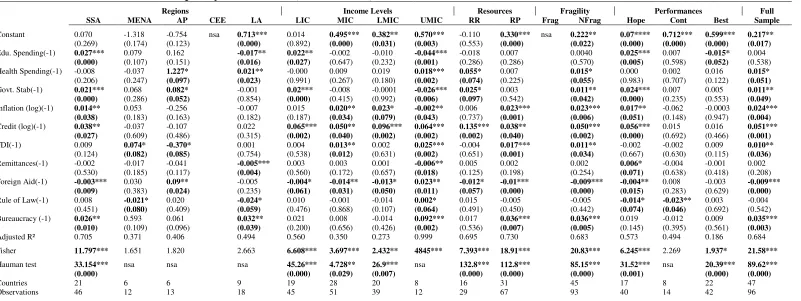
In Table 3 below showing non-contemporary OLS regressions, we have failed to
provide findings for the CEE and Fragile countries because of issues in degrees of freedom.
We use ‘nsa’ (not specifically applicable) to denote this concern. This further highlight the
issues of publication bias in social sciences raised in the introduction (Rosenberg, 2005).
12
14 Within this framework, the concern of the bias is based on strong results versus null results
(Franco et al., 1991). In what follows, we discuss the findings with particular emphasis on the
comparative element of the line of inquiry. Hence, in addition to following our simple
three-step line of interpretation, we also present comparative evidence with respect to Table 2.
The following can be established for Table 3. First, the estimated coefficients in terms
of expected signs are very heterogeneous. Second, the findings are also not broadly consistent
with the underlying paper. Third, with additional emphasis on Table 2, we compare the
estimates in chronological (or from education to bureaucracy) and increasing order of
magnitude in significance.
(i) Education spending is positively (negatively) significant for LIC, Hopefuls and
SSA (Best Performers, LA & UMIC). In relation to Table 2, Hopefuls replace Contenders in a
previously third place of positive effects; while UMIC appears in the rankings and the effect
in Best Performers is now less negative in relation to LA.
(ii) Health spending is consistently positive in: {Full Sample, NFrag}, UMIC, LA, RR
and AP. In relation to Table 2, RP and Contenders are now replaced by RR and AP. The
order of increasing positive magnitude has also changed substantially (previously: LA, RP,
UMIC, NFrag, Full Sample & Contenders).
(iii) With the exception of UMIC, government stability is positive in {NFrag, Full
Sample}, LIC, SSA, Hopefuls, RR and AP. UMIC replaces LA in the negative effect while
Contenders (RR) leaves (enters) the rankings. But the order of magnitude in significance
remains unchanged (previously, {NFrag, Full Sample}, Contenders, LIC, SSA, Hopefuls &
AP).
(iv) With the exception of UMIC, the effect of inflation is consistently positive: SSA,
15 negative (UMIC), LMIC replaces MIC while AP leaves the rankings. The corresponding
order in Table 2 was: MIC, {NFrag, Full Sample}, Hopefuls, {RP, LIC}, SSA and AP.
(v) Domestic private credit is consistently positive in {SSA, RP}, MIC, NFrag, Full
Sample, Hopefuls, UMIC, LIC, NFrag, LIMC, RR and MENA. In relation to the previous
table: the negative effect of Contenders is no longer apparent, UMIC and MIC enter into the
rankings, while the MENA leaves (previously: SSA, {RP, Hopefuls}, LIC, {NFrag, Full
Sample, LIMC}, RR and MENA).
(vi) But for AP, the effect of FDI is positive in: Full Sample, NFrag, MIC, RP, UMIC
and MENA. In relation to the contemporary findings, a substantial number of sub-panels enter
(leave) RP, UMIC & MENA (LA, LMIC, Contenders & Best Performers) the rankings. The
previous rankings are consistently positive in increasing order of: Full Sample, {LA, LMIC,
NFrag, Cont}, {Best Performers & MIC}.
(vii) The impact of remittances is now: positive in the Hopefuls and negative in LA &
UMIC, it was previously negative in LA and positive in RP, Contenders, {Hopefuls, LIC} &
UMIC.
(viii) In addition to AP, the foreign aid effect is now also positive in UMIC, and
negative in SSA, {LIC, Hopefuls}, {NFrag, Full Sample}, RP, RR, LMIC and MIC.
Hopefuls and MIC now enter into the rankings while, the impact in UMIC becomes positive.
(ix) The rule of law which was sparsely negative (in Hopefuls & Contenders) is now
more apparently negative (in Hopefuls, MENA, Contenders & LA) and positive in UMIC.
(x) Similar to the contemporary findings, the effect of bureaucratic quality is also
consistently positive with fewer sub-panels: SSA, LA, Full Sample, NFrag, RP and UMIC.
Accordingly, Hopefuls, LIC and RR leave the rankings.
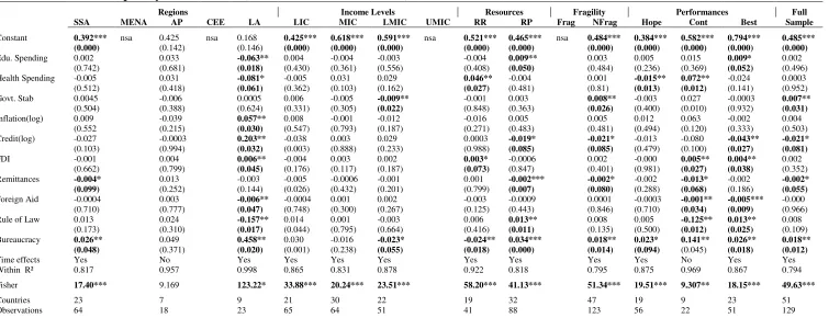
16 Due to substantial issues in degrees of freedom in the specification of some panels in
Tables 4-5, we relax the third point of the three-step line of interpretation and discuss
comparative findings of both tables simultaneously. In addition, for more subtlety in the
policy implications, we relate Tables 2-3 to the corresponding discussions in the light of how
the modeling technique actually affects the positive significance of the results. Overall, the
results substantially differ from those in Tables 2-3. This implies ‘country specific’- and
time-effects significantly influence the determinants in their time-effects on the QGI. As stated earlier,
the choice between the Fixed Effects (FE) and Random Effects (RE) model is determined by
the outcome of the Hausman test. A rejection of the null hypothesis of the underlying test
implies the FE model is a better fit. In spite of issues in degrees of freedom that have affected
some specifications and the Hausman test, we still present the available findings to mitigate
any issues of publication bias towards null findings in social sciences.
The following can be established for Tables 4-5. First, the estimated coefficients in
terms of expected signs are very heterogeneous. Second, the findings are also not broadly
consistent with the underlying paper. Third, we compare the estimates of both tables in
chronological (or from education to bureaucracy) and increasing order of magnitude in
significance.
(i) Education spending is positively (negatively) significant for Best Performers (LA).
The effects of education are more apparent in non-contemporary Fixed Effects (FE) where
they are positive in: {NFrag, Full Sample}, {LIC, LMIC}, RP, {SSA & Hopeful}.
(ii) Health spending is positive (negative) in Hopefuls & LA (RR & Contenders) while
there are no significant results in Table 5. Hence, FE modeling does not lead to positive
17 (iii) But for LMIC, government stability is positive in {NFrag, & Full Sample} and
there are no significant results in Table 5. We notice that the determinant in NFrag & Full
Sample has also been positive in Tables 2-4.
(iv) Inflation is only positive (negative) for LA (MIC) in Table 4 (5). This implies that
accounting for FE does not improve the inflation determinant because we have seen
overwhelming positive effects in Tables 2-3.
(v) But for a positive effect in LA, the impact of domestic private credit is consistently
negative in RP, {NFrag, Full Sample} & Best Performers. There are no significant results in
Table 5. This implies modeling with FE overwhelming changes the signs from positive to
negative.
(vi) FDI has positive impacts in RR, Best Performers, Contenders & LA while in
Table 5 it appears positive only for RP. Two broad policy implications results: contemporary
modeling leads to more positive effects and FE modeling should also be contemporary.
(vii) The effect of remittances is consistently negative in {RP, NFrag, Full Sample},
SSA & Contender for Table 4 and in LIC and SSA for Table 5. Overall, a change in modeling
technique and contemporary character does not substantially affect the negative effect of
remittances.
(viii) The impact of foreign aid is negative in Contenders, Best Performers & LA for
Table 4 but overwhelmingly positive in Table 5 for {RP, NFrag}, Full Sample; Hope, {SSA,
LIC} & LMIC. The fact that non-contemporary effects of foreign aid are positive implies
modeling with FE regressions has more significant and positive effects for foreign aid.
(ix) The rule of law is positive (negative) for RP & Best Performers (Contenders &
LA) and is positive for SSA in Table 5. Hence, in light of preceding tables, modeling the rule
18 (x) But for LMIC & RR that are negative, the effects of bureaucratic quality are
consistently positive for contemporary FE regressions ({NFrag, Full Sample}, Hopefuls,
{SSA, Best Performers}, RP, Contenders & LA) and only positive in for Best Performers in
the corresponding non-contemporary regressions. It follows that the latter set of regressions
with FE substantially mitigates the positive effect of this determinant that has been
overwhelming in the preceding tables.
“Insert Table 4 here”
“Insert Table 5 here”
5. Concluding implications and future research directions
We set-out to explore a new database in order to present the comparative determinants
of growth quality in 93 developing countries for the period 1990-2011. We have employed
both cross-sectional and panel estimation techniques with contemporary and
non-contemporary specifications. The empirical evidence has been based on 17 fundamental
features of growth quality derived directly and indirectly from the underlying study
motivating the inquiry (Mlachila et al., 2014). It is important to note that the impacts of the
full sample and corresponding effects on each region are not homogenous. It is essentially for
this reason that we summarize the main results in the concluding section with particular
emphasis on clarifications of such heterogeneity. In what follows, we discuss concluding
implications with emphasis on the inclusive development literature. Unless stated otherwise,
the use of ‘effect’ or ‘impact’ below technically implies the effect or impact on growth quality
across sub-panels.
We have established the following findings. First, from a cross-sectional perspective,
the four interesting results have been noticeable to elucidate complementary findings to the
19 period 2005-2011. Two factors may explain this correlation. On the one hand, “Banking
credit to the private sector in Latin America has on average increased by 7 percent of GDP
from primo 2004 to ultimo 2011, with real credit in some countries growing by up to 20
percent per year” (Hansen & Sulla, 2013, p. 1). On the other hand, relative to other regions,
Latin American countries have experienced higher levels of inequality mitigation over the
past decade (Asongu et al., 2014, p.10). (2) The positive correlation of FDI is more visible in
the periods: 1995-1999 and 2000-2004. While less visibility in the prior-1995 period could be
traceable to a substantial drop in Global FDI (Olise et al., 2013, p.1), its absence in the
post-2004 period could be explained by the recent global financial/economic crises. (3) The
negative correlation of foreign aidis not apparent during the ‘2005-2011’ interval. This may
be due to the substantial drop in official development assistance due to the 2007-2008 global
financial crises that later led to economic crisis which persisted through 2011 (Asongu,
2014b, p. 461). (4) The rule of law is negatively linked to growth quality in the initial period
(1990-1994). This could be explained by the documented U-shaped nexus between
democratisation (or governance) and economic growth in developing countries (Fosu, 2001,
p.289) and growth resurgence in Africa which was experienced only in the mid-1990s (Fosu,
2015, p.44). Overall in terms of the signs of estimated coefficients, the results broadly
confirm findings of the underlying study, with the exception of inflation (rule of law) that is
positive (negative).
Second, results based on contemporary and non-contemporary OLS are very
interesting in articulating the relevance of considering the contemporary character of
determinants. The determinants are quite heterogeneous in significance and magnitude. They
have been presented in increasing magnitude of significance so as to ease comparative
20 reproduce here for space constraint, we have enhanced readability by ensuring that the
findings are simply summarised and easy to follow.
Third, the findings of contemporary and non-contemporary panel FE have been further
compared with those of the two-preceding tables to provide policy makers with some broad
tendencies on how specification affects the outcome of the 10 determining factors. The
following have been established. (i) The positive effect of education is most apparent in
non-contemporary FE. (ii) Modelling with FE sparingly produces positive effects from health
spending. (iii) In almost all the panel models and specifications, we observe that the effects of
government stability are consistently positive in Non-Fragile states and the Full sample. (iv)
The positive effect of low and stable inflation is not very apparent with FE modelling. (v)
Specifying private domestic credit with FE overwhelming changes the sign of the
determinant from positive to negative. (vi) On the FDI determinant, one interesting
implication is noticeable: contemporary modeling results in more positive effects. (vii)
Changes in modeling technique and the contemporary specification character do not
overwhelmingly affect the negative effect of remittances. (viii) The overwhelmingly negative
effects of foreign aid become consistently positive in non-contemporary FE. (ix) Also,
modeling the rule of law with FE regressions reveals more positive results. (x) But for
non-contemporary FE regressions, the impact of bureaucratic quality is overwhelmingly positive.
In light of the above, we clarify two corresponding implications that are relevant to
policy makers: contemporary versus non-contemporary and baseline modeling versus FE
regressions. First, the contemporaneous elements of the specifications are a critical policy
direction on how to influence growth quality relative to given determinants. Accordingly, we
have observed that some determinants are positively significant when they are contemporary
than non-contemporary and vice-versa. Hence, the time-dynamic character of the
21 Second, we have also found that controlling for country- and time-effects substantially
influences signs and magnitudes of significance across specifications. Accordingly certain
variables do correlate better with time- and country-effects than others in the explanation of
growth quality.
Due to space constraints, we further discuss only the unexpected positive signs of
inflation and foreign aid which are the only determinants in the underlying study with
negative signs. First, the puzzle with inflation is the rate of inflation. Accordingly, low and
stable inflation are needed for sustainable economic growth. Monetarists term it ‘constant
inflation’ (Congdon, 2014). Stable inflation has also been documented to be favorable to
inclusive development. Albanesi (2007) has established that high inflation has a disequalizing
income-distribution impact while according to Lopez (2004) and Bulir (1998), low inflation
has the opposite effect. Second, foreign aid can be used as an instrument of inclusive human
development (Asongu & Nwachukwu, 2017d). This would require inter alia: rethinking
current development assistance models and orienting developing countries towards
industrialization according to Piketty (2014), as opposed to Kuznets’ (1955) conjectures on
the nexus between inequality and industrialization.
We set-out to present comparative determinants of growth quality. Given the
interesting results we have found, there is certainly room for more inquiries with alternative
methodologies and specification techniques. Moreover, as more data become available,
estimation approaches that account for the dynamic character of growth quality like the
Generalised Method of Moments (GMM) are worthwhile. This is essentially because at least
five data points are needed to employ the GMM. Unfortunately, the dataset is based on four
22
Table 1: Cross sectional regressions (Contemporary determinants)
90-94 95-99 00-04 05-11 90-94 95-99 00-04 05-11
Without Heteroscedasticity Consistency With Heteroscedasticity Consistency
Constant 0.221 0.442** 0.381*** 0.145 0.221 0.442*** 0.381** 0.145 (0.398) (0.020) (0.000) (0.365) (0.439) (0.000) (0.020) (0.510)
Edu. Spending 0.004 0.015 0.003 0.001 0.004 0.015 0.003 0.001
(0.916) (0.151) (0.710) (0.907) (0.911) (0.136) (0.700) (0.892)
Health Spending 0.067 0.003 0.002 0.024 0.067 0.003 0.002 0.024
(0.220) (0.819) (0.819) (0.145) (0.245) (0.761) (0.753) (0.188)
Govt. Stab 0.029 -0.014 -0.005 0.001 0.029 -0.014 -0.005 0.001
(0.251) (0.505) (0.683) (0.886) (0.293) (0.407) (0.695) (0.907) Inflation (log) 0.052 0.036** 0.019 0.008 0.052 0.036** 0.019 0.008
(0.260) (0.016) (0.218) (0.796) (0.340) (0.020) (0.223) (0.848)
Credit (log) 0.027 0.019 0.026 0.081* 0.027 0.019 0.026 0.081***
(0.721) (0.476) (0.196) (0.056) (0.729) (0.460) (0.198) (0.007)
FDI -0.037 0.019** 0.010* -0.002 -0.037 0.019*** 0.010*** -0.002
(0.305) (0.012) (0.063) (0.659) (0.365) (0.001) (0.000) (0.669) Remittances 0.014 0.005 0.005** -0.002 0.014 0.005 0.005** -0.002
(0.172) (0.124) (0.033) (0.582) (0.197) (0.100) (0.035) (0.512) Foreign Aid -0.011** -0.016*** -0.014*** -0.005 -0.011* -0.016*** -0.014*** -0.005
(0.042) (0.000) (0.000) (0.275) (0.069) (0.000) (0.000) (0.138)
Rule of Law -0.097* -0.002 0.009 0.017 -0.097* -0.002 0.009 0.017
(0.061) (0.834) (0.362) (0.413) (0.057) (0.807) (0.338) (0.339)
Bureaucracy 0.059* 0.041* 0.060*** 0.062** 0.059** 0.041** 0.060*** 0.062***
(0.084) (0.059) (0.006) (0.026) (0.047) (0.015) (0.003) (0.005)
Adjusted R² 0.658 0.823 0.693 0.517 0.658 0.823 0.693 0.517
Fisher 4.664** 15.95*** 10.52*** 4.435*** 6.407*** 25.80*** 28.297*** 8.019***
Observations 20 60 43 33 20 60 43 33
23
Table 2: Baseline contemporary determinants (HAC SE OLS)
Regions Income Levels Resources Fragility Performances Full
SSA MENA AP CEE LA LIC MIC LMIC UMIC RR RP Frag NFrag Hope Cont Best Sample
Constant 0.029 0.353 0.080 nsa 0.710*** -0.022 0.396*** 0.345* 0.129 -0.028 0.225*** nsa 0.133 0.085 0.536*** 0.651*** 0.137 (0.610) (0.153) (0.720) (0.000) (0.804) (0.006) (0.053) (0.346) (0.833-) (0.000) (0.163) (0.295) (0.000) (0.000) (0.141) Edu. Spending 0.016** -0.0004 0.015 -0.008* 0.014** -0.010 -0.014 -0.035 -0.010 0.0008 -0.001 0.012 0.017*** -0.014** -0.0006
(0.014) (0.978) (0.699) (0.055) (0.029) (0.146) (0.106) (0.129) (0.376) (0.901) (0.846) (0.070) (0.000) (0.032) (0.920) Health Spending 0.001 0.0307 0.073 0.012* 0.007 0.015 0.020 0.015** 0.030 0.014** 0.019** -0.0006 0.022** 0.013 0.019**
(0.818) (0.113) (0.225) (0.060) (0.382) (0.102) (0.141) (0.025) (0.215) (0.049) (0.013) (0.879) (0.016) (0.131) (0.011)
Govt. Stab 0.023*** -0.009 0.04** -0.006** 0.017*** 0.001 0.004 0.014 0.014 0.007 0.012* 0.024*** 0.014** 0.001 0.012** (0.000) (0.579) (0.013) (0.030) (0.000) (0.841) (0.683) (0.423) (0.275) (0.111) (0.053) (0.000) (0.012) (0.804) (0.048)
Inflation (log) 0.030*** -0.004 0.094** -0.003 0.029*** 0.019* 0.023 0.033 -0.014 0.029*** 0.023** 0.025*** -0.018 -0.003 0.023** (0.000) (0.869) (0.019) (0.337) (0.009) (0.092) (0.152) (0.112) (0.478) (0.000) (0.032) (0.002) (0.144) (0.555) (0.022)
Credit (log) 0.036*** 0.155** -0.027 -0.014 0.058*** 0.043 0.068* 0.040 0.118*** 0.041*** 0.058*** 0.041*** -0.027** 0.011 0.058*** (0.002) (0.037) (0.544) (0.458) (0.001) (0.116) (0.077) (0.229) (0.000) (0.007) (0.000) (0.000) (0.019) (0.535) (0.000)
FDI 0.0004 0.011 -0.017 0.006*** 0.001 0.008*** 0.006** 0.010 0.0007 0.003 0.006** -0.002 0.006** 0.008** 0.005*
(0.863) (0.203) (0.199) (0.002 (0.779 (0.001) (0.026) (0.209) (0.861) (0.381) (0.046) (0.343) (0.015) (0.012) (0.067)
Remittances 0.004 -0.000 -0.004 -0.003*** 0.008** 0.0001 -0.001 0.024* 0.007 0.003* 0.002 0.008*** 0.005*** -0.001 0.002 (0.135) (0.994) (0.283) (0.003) (0.025) (0.925) (0.689) (0.097) (0.143) (0.080) (0.362) (0.001) (0.000) (0.203) (0.266) Foreign Aid -0.006*** -0.022 0.027** -0.005 -0.006*** -0.006 -0.008* -0.031* -0.014*** -0.009*** -0.009*** -0.005*** -0.002 -0.004 -0.009***
(0.000) (0.207) (0.054) (0.118) (0.000) (0.123) (0.072) (0.090) (0.001) (0.000) (0.000) (0.000) (0.141) (0.283) (0.000)
Rule of Law 0.007 -0.013 -0.001 -0.001 0.014 -0.0003 -0.003 -0.008 0.028 -0.001 -0.002 -0.015*** -0.021*** 0.007 -0.001 (0.444) (0.280) (0.962) (0.828) (0.241) (0.966) (0.700) (0.564) (0.150) (0.778) (0.736) (0.003) (0.000) (0.413) (0.809) Bureaucracy 0.036*** -0.122 0.034 0.053*** 0.037*** 0.028 0.010 0.134*** 0.044* 0.048*** 0.056*** 0.031**** 0.013 0.001 0.051***
(0.000) (0.183) (0.347) (0.000) (0.001) (0.150) (0.662) (0.006) (0.051) (0.000) (0.000) (0.003) (0.242) (0.932) (0.000)
Adjusted R² 0.741 0.152 0.547 0.776 0.711 0.275 0.165 0.477 0.726 0.730 0.690 0.707 0.751 0.185 0.688 Fisher 19.055*** 1.270 0.945 8.659*** 16.778*** 3.396*** 1.990* 2.098 11.61*** 24.60*** 28.16*** 14.29*** 7.353*** 2.139** 29.23***
Hauman test 17.015** n.s.a nsa nsa 59.82*** 27.31*** 16.837 nsa 327.9*** 82.17*** 90.45*** 50.04*** nsa 24.86** 93.72***
(0.074) (0.000) (0.000) (0.206) (0.000) (0.000) (0.000) (0.000) (0.024) (0.000)
Countries 23 7 7 9 21 30 22 8 19 32 47 19 9 23 51
Observations 64 16 18 23 65 64 51 13 41 88 123 56 22 51 129
24
Table 3: Baseline non-contemporary determinants (HAC SE OLS)
Regions Income Levels Resources Fragility Performances Full
SSA MENA AP CEE LA LIC MIC LMIC UMIC RR RP Frag NFrag Hope Cont Best Sample
Constant 0.070 -1.318 -0.754 nsa 0.713*** 0.014 0.495*** 0.382** 0.570*** -0.110 0.330*** nsa 0.222** 0.07**** 0.712*** 0.599*** 0.217**
(0.269) (0.174) (0.123) (0.000) (0.892) (0.000) (0.031) (0.003) (0.553) (0.000) (0.022) (0.000) (0.000) (0.000) (0.017)
Edu. Spending(-1) 0.027*** 0.079 0.162 -0.017** 0.022** -0.002 -0.010 -0.044*** -0.018 0.007 0.0040 0.025*** 0.007 -0.015* 0.004
(0.000) (0.107) (0.151) (0.016) (0.027) (0.647) (0.232) (0.001) (0.286) (0.286) (0.570) (0.005) (0.598) (0.052) (0.538) Health Spending(-1) -0.008 -0.037 1.227* 0.021** -0.000 0.009 0.019 0.018*** 0.055* 0.007 0.015* 0.000 0.002 0.016 0.015*
(0.206) (0.247) (0.097) (0.023) (0.991) (0.267) (0.180) (0.002) (0.074) (0.225) (0.055) (0.983) (0.707) (0.122) (0.051)
Govt. Stab(-1) 0.021*** 0.068 0.082* -0.001 0.02*** -0.008 -0.0001 -0.026*** 0.025* 0.003 0.011** 0.024*** 0.007 0.005 0.011** (0.000) (0.286) (0.052) (0.854) (0.000) (0.415) (0.992) (0.006) (0.097) (0.542) (0.042) (0.000) (0.235) (0.553) (0.049)
Inflation (log)(-1) 0.014** 0.053 -0.256 -0.007 0.015 0.020** 0.023* -0.002** 0.006 0.023*** 0.023*** 0.017** -0.062 -0.0003 0.024*** (0.038) (0.183) (0.163) (0.182) (0.187) (0.034) (0.079) (0.043) (0.737) (0.001) (0.006) (0.051) (0.148) (0.947) (0.004)
Credit (log)(-1) 0.038** -0.037 -0.107 0.022 0.065*** 0.050** 0.096*** 0.064*** 0.135*** 0.038** 0.050*** 0.056*** 0.015 0.016 0.051*** (0.027) (0.609) (0.486) (0.315) (0.002) (0.040) (0.002) (0.002) (0.002) (0.040) (0.002) (0.000) (0.692) (0.466) (0.001)
FDI(-1) 0.009 0.074* -0.370* 0.001 0.004 0.013** 0.002 0.025*** -0.004 0.017*** 0.011** -0.002 -0.002 0.009 0.010**
(0.124) (0.082) (0.085) (0.754) (0.538) (0.012) (0.631) (0.002) (0.651) (0.001) (0.034) (0.667) (0.630) (0.115) (0.036)
Remittances(-1) -0.002 -0.017 -0.041 -0.005*** 0.003 0.003 0.001 -0.006** 0.005 0.002 0.002 0.006* -0.004 -0.001 0.002 (0.530) (0.185) (0.117) (0.004) (0.560) (0.172) (0.657) (0.018) (0.125) (0.198) (0.254) (0.071) (0.638) (0.418) (0.208) Foreign Aid(-1) -0.003*** 0.030 0.09** -0.005 -0.004* -0.014** -0.013* 0.023** -0.012* -0.01*** -0.009*** -0.004** 0.008 -0.003 -0.009***
(0.009) (0.383) (0.024) (0.235) (0.061) (0.031) (0.050) (0.011) (0.057) (0.000) (0.000) (0.015) (0.283) (0.629) (0.000)
Rule of Law(-1) 0.008 -0.021* 0.020 -0.024* 0.010 -0.001 -0.014 0.002* 0.015 -0.005 -0.005 -0.014* -0.023** 0.003 -0.004 (0.451) (0.080) (0.409) (0.059) (0.476) (0.868) (0.107) (0.064) (0.491) (0.450) (0.442) (0.074) (0.046) (0.692) (0.542) Bureaucracy (-1) 0.026** 0.593 0.061 0.032** 0.021 0.008 -0.014 0.092*** 0.017 0.036*** 0.036*** 0.019 -0.012 0.009 0.035***
(0.010) (0.109) (0.096) (0.039) (0.200) (0.656) (0.426) (0.002) (0.536) (0.007) (0.005) (0.145) (0.395) (0.561) (0.003)
Adjusted R² 0.705 0.371 0.406 0.494 0.560 0.350 0.273 0.999 0.695 0.730 0.683 0.573 0.494 0.186 0.684 Fisher 11.797*** 1.651 1.820 2.663 6.608*** 3.697*** 2.432** 4845*** 7.393*** 18.91*** 20.83*** 6.245*** 2.269 1.937* 21.58***
Hauman test 33.154*** nsa nsa nsa 45.26*** 4.728** 26.9*** nsa 132.8*** 112.8*** 85.15*** 31.52*** nsa 20.39*** 89.62***
(0.000) (0.000) (0.029) (0.007) (0.000) (0.000) (0.000) (0.001) (0.000) (0.000)
Countries 21 6 6 9 19 28 20 8 16 31 45 17 8 22 47
Observations 46 12 13 18 45 51 39 12 29 67 93 40 14 42 96
25
Table 4: Contemporary determinants (HAC SE Panel Fixed effects)
Regions Income Levels Resources Fragility Performances Full
SSA MENA AP CEE LA LIC MIC LMIC UMIC RR RP Frag NFrag Hope Cont Best Sample
Constant 0.392*** nsa 0.425 nsa 0.168 0.425*** 0.618*** 0.591*** nsa 0.521*** 0.465*** nsa 0.484*** 0.384*** 0.582*** 0.794*** 0.485*** (0.000) (0.142) (0.146) (0.000) (0.000) (0.000) (0.000) (0.000) (0.000) (0.000) (0.000) (0.000) (0.000)
Edu. Spending 0.002 0.033 -0.063** 0.004 -0.004 -0.003 -0.004 0.009** 0.003 0.005 0.015 0.009* 0.002 (0.742) (0.681) (0.018) (0.430) (0.361) (0.556) (0.408) (0.050) (0.484) (0.236) (0.369) (0.052) (0.496) Health Spending -0.005 0.031 -0.081* -0.005 0.031 0.029 0.046** -0.004 0.001 -0.015** 0.072** -0.024 0.0003 (0.512) (0.418) (0.061) (0.362) (0.103) (0.162) (0.027) (0.481) (0.81) (0.013) (0.012) (0.141) (0.952) Govt. Stab 0.0045 -0.006 0.0005 0.006 -0.005 -0.009** -0.001 0.003 0.008** -0.003 0.027 -0.0003 0.007**
(0.504) (0.388) (0.624) (0.331) (0.305) (0.022) (0.848) (0.363) (0.026) (0.400) (0.010) (0.932) (0.031)
Inflation(log) 0.009 -0.039 0.057** 0.008 -0.001 -0.012 -0.016 0.005 0.005 0.012 0.063 -0.002 0.004 (0.552 (0.215) (0.030) (0.547) (0.793) (0.187) (0.271) (0.483) (0.481) (0.494) (0.120) (0.333) (0.503) Credit(log) -0.027 -0.0003 0.203** -0.038 0.003 0.029 0.0003 -0.019* -0.021* -0.013 -0.080 -0.043** -0.021*
(0.103) (0.994) (0.032) (0.003) (0.888) (0.233) (0.988) (0.085) (0.085) (0.479) (0.100) (0.027) (0.081)
FDI -0.001 0.004 0.006** -0.004 0.003 0.002 0.003* -0.0006 0.002 -0.000 0.005** 0.004** 0.002 (0.662) (0.799) (0.045) (0.176) (0.117) (0.187) (0.073) (0.847) (0.401) (0.981) (0.027) (0.038) (0.352) Remittances -0.004* 0.013 -0.003 -0.005 -0.0006 -0.001 0.001 -0.002*** -0.002* -0.002 -0.013* -0.002 -0.002* (0.099) (0.252) (0.144) (0.026) (0.432) (0.201) (0.799) (0.007) (0.080) (0.288) (0.068) (0.186) (0.055)
Foreign Aid -0.0004 0.003 -0.006** -0.0004 0.001 0.002 -0.003 -0.0009 0.0001 -0.0003 -0.001** -0.005*** -0.000 (0.710) (0.777) (0.047) (0.748) (0.300) (0.267) (0.125) (0.443) (0.846) (0.710) (0.034) (0.009) (0.966) Rule of Law 0.013 0.024 -0.157** 0.014 0.001 -0.003 0.006 0.013** 0.008 0.005 -0.125** 0.013** 0.008
(0.173) (0.310) (0.017) (0.044) (0.795) (0.664) (0.416) (0.011) (0.135) (0.500) (0.012) (0.025) (0.109) Bureaucracy 0.026** 0.049 0.458** 0.030 -0.016 -0.023* -0.024** 0.034*** 0.018** 0.023* 0.141** 0.026** 0.018**
(0.048) (0.371) (0.020) (0.001) (0.238) (0.055) (0.018) (0.000) (0.014) (0.094) (0.045) (0.018) (0.012)
Time effects Yes No Yes Yes Yes Yes Yes Yes Yes Yes No Yes Yes Within R² 0.817 0.957 0.998 0.865 0.831 0.878 0.922 0.818 0.795 0.875 0.969 0.867 0.794 Fisher 17.40*** 9.169 123.22* 33.88*** 20.24*** 23.51*** 58.20*** 41.13*** 51.34*** 19.51*** 9.307** 18.15*** 49.63***
Countries 23 7 9 21 30 22 19 32 47 19 9 23 51
Observations 64 18 23 65 64 51 41 88 123 56 22 51 129
26
Table 5: Non-contemporary determinants (HAC SE Panel Fixed effects)
Regions Income Levels Resources Fragility Performances Full
SSA MENA AP CEE LA LIC MIC LMIC UMIC RR RP Frag NFrag Hope Cont Best Sample
Constant 0.389*** nsa nsa nsa nsa 0.406*** 0.643*** 0.912*** nsa 2.019 0.458*** nsa 0.561*** 0.31*** nsa 0.646*** 0.513***
(0.000) (0.000) (0.000) (0.001) (0.124) (0.000) (0.000) (0.000) (0.000) (0.000)
Edu. Spending(-1) 0.019*** 0.015** 0.001 0.015* -0.008 0.016*** 0.011** 0.019*** -0.002 0.011***
(0.003) (0.011) (0.742) (0.060) (0.422) (0.000) (0.011) (0.005) (0.677 (0.006)
Health Spending(-1) 0.002 -0.000 0.020 -0.001 0.267 0.003 0.003 -0.0005 0.027 0.004
(0.680) (0.997) (0.187) (0.942) (0.118) (0.410) (0.487) (0.923) (0.174) (0.400)
Govt. Stab(-1) -0.007 0.002 -0.001 0.003 -0.060 0.006 0.006 -0.005 -0.004 0.006
(0.392) (0.747) (0.736) (0.590) (0.122) (0.183) (0.135) (0.445) (0.549) (0.130)
Inflation(-1)(log) -0.004 -0.002 -0.009*** -0.001 0.297 -0.0009 -0.003 -0.005 -0.006 -0.002
(0.751) (0.845) (0.005) (0.945) (0.119) (0.850) (0.512) (0.764) (0.064) (0.552)
Credit(-1)(log) -0.016 -0.021 -0.002 -0.116 -0.671 0.0003 -0.013 0.015 0.029 -0.014
(0.454) (0.260) (0.914) (0.210) (0.160) (0.984) (0.407) (0.474) (0.221) (0.361)
FDI(-1) 0.005 0.012 -0.005 -0.0004 0.028 0.009* 0.0009 0.006 -0.0002 0.0008
(0.378) (0.107) (0.054) (0.875) (0.208) (0.092) (0.807) (0.348) (0.928) (0.826)
Remittances(-1) -0.007** -0.006** 0.001 -0.0003 -0.115 -0.003 -0.002 -0.002 0.001 -0.002
(0.032) (0.048) (0.262) (0.881) (0.101) (0.171) (0.383) (0.541) (0.318) (0.271)
Foreign Aid(-1) 0.005*** 0.005*** 0.009 0.007* -0.044 0.002** 0.002* 0.004*** 0.005 0.003*
(0.003) (0.002) (0.080) (0.093) (0.156) (0.045) (0.078) (0.007) (0.190) (0.068)
Rule of Law(-1) 0.024* 0.007 0.010 0.027 0.140 0.011* 0.012 0.006 0.003 0.011
(0.057) (0.478) (0.204) (0.192) (0.142) (0.093) (0.163) (0.634) (0.430) (0.176)
Bureaucracy (-1) -0.008 -0.002 -0.016 0.009 0.015 0.005 -0.007 0.0002 -0.020* -0.006
(0.538) (0.849) (0.147) (0.587) (0.527) (0.384) (0.474) (0.980) (0.065) (0.504)
Time effects Yes Yes Yes Yes Yes Yes Yes Yes Yes Yes
Within R² 0.877 0.901 0.781 0.758 0.937 0.872 0.766 0.879 0.898 0.765
Fisher 18.19*** 29.16*** 17.77*** 12.33*** 16.2*** 52.42*** 42.25*** 13.18*** 18.69*** 41.97***
Countries 21 19 28 20 16 31 45 17 22 47
Observations 46 45 51 39 29 67 93 40 42 96
27
Appendices
Appendix 1: Definition of variables
Variable(s) Definition(s) Source(s)
Quality of Growth Index (QGI)
“Composite index ranging between 0 and 1, resulting from the
aggregation of components capturing growth fundamentals and from components capturing the socially-friendly nature of growth. The higher the index, the greater is the quality of growth” (p. 25).
Mlachila et al. (2014)
Educational Spending
“Public resources allocated to education spending, as percent of GDP” (p. 25)
Mlachila et al. (2014)
Health Spending “Public resources allocated to heath spending, as percent of GDP” (p.
25)
Mlachila et al. (2014)
Government Stability
“Index ranging from 0 to 12 and measuring the ability of government to stay in office and to carry out its declared program(s).The higher the index, the more stable the government is” (p. 25).
Mlachila et al. (2014)
Inflation Inflation rate based on the Consumer Price Index (CPI) Mlachila et al.
(2014)
Credit to private sector
“Domestic credit to private sector, namely credit offered by the banks to the private sector, as percent of GDP” (p. 25).
Mlachila et al. (2014)
Foreign Direct Investment
“Net Inflows of Foreign Direct Investments, as percent of GDP” (p. 25) Mlachila et al.
(2014)
Remittances
“Workers' remittances and compensation of employees (Percent of
GDP), calculated as the sum of workers' remittances, compensation of employees and migrants' transfers” (p. 25).
Mlachila et al. (2014)
Foreign Aid “Official development Aid actually disbursed, as percent of GDP” (p.
25)
Mlachila et al. (2014)
Rule of Law
“Index assessing the strength and the impartiality of the legal system, as well as the popular observance of the law. The index ranges from 0 to 6, with a higher value of the index reflecting a higher institutional Quality” (p. 25).
Mlachila et al. (2014)
Quality of Bureaucracy
“Index of the institutional strength and quality of the bureaucracy, ranging from 0 to 4. The higher the index, the stronger the quality of the bureaucracy” (p. 25)
Mlachila et al. (2014)
Appendix 2: Summary Statistics
Mean S. D Minimum Maximum Obs
Quality of Growth Index (QGI) 0.604 0.140 0.258 0.849 372
Educational Spending 0.612 0.263 0.000 1.000 372
Health Spending 0.676 0.208 0.089 0.995 372
Government Stability 18.518 165.55 2.666 2873.8 303
Inflation (log) 2.331 1.358 -0.637 8.767 339
Domestic Credit (log) 3.355 0.798 0.529 5.131 345
Foreign Direct Investment 3.225 4.867 -4.172 62.264 366
Remittances 4.117 7.391 0.001 63.295 322
Foreign Aid 4.921 5.771 -9.546 36.317 226
Rule of Law 3.290 1.060 0.666 5.933 301
Quality of Bureaucracy 1.693 0.772 0.000 4.000 301
28
Appendix 3: Correlation Matrix
Educ Health GovStab Infl(log) Credit(log) FDI Remit Aid Law Bureau QGI
1.000 0.594 0.024 -0.007 0.152 0.048 0.419 -0.014 0.219 0.214 0.098 Educ
1.000 0.036 0.032 0.231 0.133 0.265 -0.070 0.214 0.228 0.340 Health
1.000 -0.002 -0.007 -0.050 -0.046 0.160 0.355 0.025 -0.119 GovStab
1.000 -0.103 -0.111 -0.058 0.088 -0.100 -0.071 -0.003 Infl(log)
1.000 -0.047 -0.018 -0.230 0.235 0.464 0.551 Credit(log)
1.000 0.134 -0.062 0.130 -0.069 0.038 FDI
1.000 -0.027 -0.040 -0.058 -0.033 Remit
1.000 -0.059 -0.304 -0.572 Aid
1.000 0.256 0.352 Law
1.000 0.493 Bureau QGI
Educ: Educational Spending. Health: Health Spending. GovStab: Government Stability. Infl: Inflation. Credit: Domestic Credit. FDI: Foreign Direct Investment. Remit: Remittances. Aid: Foreign Aid. Law: Rule of Law. Bureau: Bureaucracy. QGI: Quality of Growth Index.
References
Alan, K., & Carlyn, R-D., (2015). “Is Africa Actually Developing?”, World Development, 66(C), pp. 598-613.
Allen, K., (2014). “Review: Thomas Piketty, Capital in the Twenty First Century”, Irish Maxist Review, 3(10)
Amavilah, V. H. S., (2014). “Sir W. Arthur Lewis and the Africans: Overlooked Economic Growth Lessons”, MPRA Paper No. 57126, Munich.
Anand, R., Mishra, S., & Peiris, S. J., (2013). “Inclusive Growth: Measurement and
Determinants”, IMF Working Paper 13/135, Washington.
Anand, R., Mishra, S., & Spatafora, N., (2012), “Structural Transformation and
the Sophistication of Production,” IMF Working Paper No. 12/59, Washington.
Anyanwu, J. C., (2014a). “Marital Status, Household Size and Poverty in Nigeria: Evidence
from the 2009/2010 Survey Data”, African Development Review, 26(1), pp. 118-137.
Anyanwu, J. C., (2014b). “Determining the correlates of poverty for inclusive growth in
Africa”, European Economics Letters, 3(1), pp. 12-17.
Anyanwu, J. C., (2013a). “Gender Equality in Employment in Africa: Empirical Analysis and Policy Implications”, African Development Review, 25(4), pp. 400-420.
Anyanwu, J. C., (2013b). “The correlates of poverty in Nigeria and policy implications”,
African Journal of Economic and Sustainable Development, 2(1), pp. 23-52.