Munich Personal RePEc Archive
Addressing multicollinearity in regression
models: a ridge regression application
Bager, Ali and Roman, Monica and Algedih, Meshal and
Mohammed, Bahr
Bucharest University of Economic Studies, Bucharest University of
Economic Studies, Bucharest University of Economic Studies,
Bucharest University of Economic Studies
June 2017
Online at
https://mpra.ub.uni-muenchen.de/81390/
ADDRESSING MULTICOLLINEARITY IN REGRESSION MODELS:
A RIDGE REGRESSION APPLICATION
1Ali BAGERa, Monica ROMANb, Meshal ALGELIDHc, Bahr MOHAMMEDd
Abstract
The aim of this paper is to determine the most important macroeconomic factors which affect the unemployment rate in Iraq, using the ridge regression method as one of the most widely used methods for solving the multicollinearity problem. The results are compared with those obtained with the OLS method, in order to produce the best possible model that expresses the studied phenomenon. After applying indicators such as the condition number (CN) and the variance inflation factor (VIF) in order to detect the multicollinearity problem and after using R packages for simulations and computations, we have proven that in Iraq, as an Arabic developing economy, unemployment seems to be significantly affected by investments, working population size and inflation.
Keywords: multicollinearity, ridge regression method, unemployment rate.
JEL Classification : C51, C12, J64
Authors’ Affiliation
a
-The Bucharest University of Economic Studies, Doctoral School and Muthanna University, corresponding author, [email protected]
b
-The Bucharest University of Economic Studies, Department of Statistics and Econometrics
c
-The Bucharest University of Economic Studies, Doctoral School and Muthanna University
d
-The Bucharest University of Economic Studies, Doctoral School and University of AL-Qadisiyah
1
2
1. Introduction
The countries in the world, in general, and the Arab countries in particular, are affected by labor market imbalances and unemployment, the magnitude of this depending on the nature of the economic system and the degree of economic development. In Iraq, the financial crisis has contributed to an increase in unemployment and has taken its toll on the living standard. Since mid-2014, Iraq has been experiencing a severe economic and financial crisis that has begun to escalate and exacerbate for objective and subjective reasons, including: financial mismanagement and financial and administrative corruption in the state owned economic institutions, in the context of the severe fall by up to 65% of the oil price on the world markets. It should be noted that Iraq relies entirely on oil resources and not on development plans and programs to diversify its resources and encourage other economic sectors such as agriculture, industry, tourism, etc. The decrease in oil prices has reduced the liquidity of the country and has had a clear impact on the society by raising the unemployment rate and the poverty level. Its negative effects are also seen in the delivery of services in the areas of health and education and even in the infrastructure.
Although the literature on the Iraqi economic development is not very generous, there are studies that have tackled this issue. In 2013, Shammari studied the trends and causes of unemployment in Iraq after 2003. The study was aimed to identify ways and means of dealing with unemployment and its effects and concluded that due to the economic policies, between 2003 and 2008 the unemployment rate had gone down from 28.10% to 15.34%. This decrease, though important, is still insufficient in the context of the Iraqi economy, since there is a high number of job seekers because of the high population growth.
3
When using multiple linear regressions at macro level, researchers can face many problems, including multicollinearity. This problem arises because of the high correlation between the independent variables that lead to weak estimates.
In his work in 1934, Fisher was among the first researchers who indicated the seriousness of the multicollinearity problem and its effect on the results of the regression analysis. Following that, many researchers have pursued the different aspects and ways of solving this issue. In 1975, Hoerl and Kennard developed a new method by adding a positive value to the elements of the information matrix (X' X), the so called biased parameter and the ridge regression method.
An iterative method for choosing the value of the parameter k was developed by Hoerl and Kennard (1976) Montgomery and Peck (1982) proved that the ridge trace depends on the path of the estimated curves versus a number of constant values between zero and one. In 1965, Massy presented a study that included the use of the standard ridge regression method to address the multicollinearity problem in linear regression by finding a new estimator for the regression coefficients that have less variance than those of the variance of least squares.
In 2010, AL-Hassan used the ridge regression as an alternative to the ordinary least square method of estimation when there is multi-linearity between explanatory variables. The researcher also proposed a new method for choosing the ridge parameter and used simulation data to evaluate the performance of the proposed method, by using the mean square error (MSE) to compare estimations. In 2014, Fitrianto and Yik reported that when a linear correlation between the explanatory variables of the multiple linear regression models is high, the variance is higher than in the case of the OLS method. The researchers used the ridge regression study to compare the performance of the ridge regression estimator and OLS, confirming that Hoerl & Kennard's ridge regression method had a better performance than other methods.
The aim of this paper is to test the performance of the ridge regression estimators, when the data used in the model refers to macro-economic indicators. In many cases, these indicators are subject to multicollinearity. The paper would also contribute to the existing literature by offering new insights into the macroeconomic determinants of unemployment in Iraq.
4
ridge regression method and in Section 5 we use the ridge regression method on sample data. The conclusions of the study are presented in the final section.
2. General linear regression model
There is a large variety of regression models (i.e. simple, linear, non-linear) and their use depends on the specific type of problem that is studied. Multiple regression models are used when the response variable Y depends on a set of explanatory variables (X1, X2, … , Xm). The phenomena in economy and society are complex and usually require more than one explanatory variable to be analyzed and understood. Therefore, in order to determine the effects on a dependent variable, one of the most common approaches is the multilinear regression model, which is also applied in this research.
The linear regression model is defined by a dependent variable (Y) explained through
a set of multiple explanatory variables (
X
j)
and it is based on the assumption that there is alinear relationship between the explained variable (
Y
i)and the explanatory variables(
x
1, x
2. x
3, … , x
m). Random error(Ƹ
i)
is associated with each of theobservations(Yi), (i = 1,2, … , n), as a linear function in the explanatory set
(xi1, xi2, xi3, … , xim), as follows:
Yi = β0+ β1X1i+ β2X1i+ ⋯ + βmXim+ ƹi (1)
and:
i = 1,2, … , n , j = 0,1,2, … , m ,
X0 = 1
β
0, β
1, … , β
m: Represent the parameters of the regression.ƹ
i: Represent random errors.The model can be written briefly as follows:
Y
i= ∑ β
jX
ij+ ƹ
i(2)
mj=0
Using the matrix form, the above equation can be formalized as follows:
5
[
Y
1Y
2⋮
Y
n] = [
1
1
⋮
1
x
11x
21⋮
x
n1x
12x
22⋮
x
n2…
…
⋱
…
x
1mx
2m⋮
x
nm] [
β
0β
1⋮
β
m] + [
ƹ
1ƹ
2⋮
ƹ
n] (3)
Where:
Y
:
a vector of the class (n × 1) which represents the values of the variable response;X
:
The matrix of the class (n × (m + 1)) that represents the observations of the explanatory variables;β
:
Vector of the parameters to be estimated, from the ((m + 1) × 1)class;ƹ
:
Random errors vector, of (n × 1)class;The linear regression model relies on a set of hypotheses, including multicollinearity, as follows:
- Random errors are normally distributed:
ƹ
i~ N(0, σ
2I
n)
- Different values for random error (ƹi)tsumbe independent:
-Cov(ƹiƹj) = E(ƹi ƹj) = 0 ∀ i ≠ j
- The values of random errors (ƹi)are not associated with any of the explanatory variables:
E(ƹixi) = 0
- The explanatory variables are not linked to each other by a complete or almost complete linear relationship; in addition, the number of parameters to be estimated should be less than the size of the sample under research.
cov(x
i, x
j) = 0 ∀ i ≠ j
Rank (X) = m + 1 < 𝑛
6
3. Multicollinearity problem
The multicollinearity problem is defined as the association between two or more explanatory variables through a strong linear relationship in which the effect of the dependent variables cannot be separated from that of the explanatory variables. The problem of linear
multicollinearity is also described through the concept of “orthogonality”: when the explanatory variables are orthogonal (not linked to each other), all the eigen values are equal to one; if one of these eigen values is less than one, especially when it is equal to or near zero, than it is not orthogonal, leading to the problem of linear multicollinearity.
Linear multicollinearity is considered to be of two types:
The Prefect Multicollinearity: In this type of linear multicollinearity, the specific matrix of information (XX́) has a determinant equal to zero (|XX́| = 0) and thus we cannot find the estimators of the general linear regression model since it is not possible to find the inverse matrix.
Semi Multicollinearity: It is the subject of the research in which the value of a specific determinant of the matrix of information (XX́) is very small and close to zero: |XX́| ≈ 0. Thefore, the estimators of the parameters can be found, but the consequence of this type of multicollinearity is that estimates are inaccurate, and the estimated differences in parameters are very large.
3.1. Detecting multicollinearity in regression models
3.1.1. Condition Number
The Condition number (CN) is a measure proposed for detecting the existence of the multicollinearity in regression models. This measure is based on the eigen values of the explanatory variable matrix, measuring the sensitivity of regression estimators to small variations in variances.
CN is computed using the following formula:
C. N = √
λ
λ
maxmin
(4)
7
λmin the smallest eigenvalue for the matrix XX́
If the CN is between 20 and 30, this is an indicator for a high linear multicollinearity. Some researchers, such as Yong-wei (2008), suggested that when the CN is between 30 and 100, this is a sign of very high linear multicollinearity.
3.1.2. Variance Inflation Factor
Proposed by Farrar and Glauber in 1967, the Variance Inflation Factor (VIF) measures the inflation of the parameter estimates being computed for all explanatory variables in the model.
The VIF formula is as follows:
VIF =
1
1 − R
2j, j = 0,1,2, … , m (5)
where Rj2 is the Coefficient of Determination for the explanatory variable .
The coefficient of determination ranges between 0 and 1 and is calculated in the case of four explanatory variables according to the following formula:
𝑅
𝑗2= 1 − (1 − 𝑟
122)(1 − 𝑟
12.32)(1 − 𝑟
14.232) (6)
where: 𝑟122 represents the simple correlation coefficient and 𝑟12.32 𝑎𝑛𝑑 𝑟14.232 represent the partial correlation coefficients.
In this research, VIF is calculated for each explanatory variable and it is used to assess the correlation of each explanatory variable with the other variables in the model. When the value of the coefficient of determination Rj2 is close to or equal to one, it indicates the
presence of multicollinearity between explanatory variables, which makes the value of VIF large. On the other hand, when the variable Xj is independent of the rest of the other
explanatory variables, the value of the coefficient of determination is
R2j = 0 and this leads to: VIF=1
8
4. Ridge regression method
In order to estimate the parameters of the linear regression model in the case of multicollinearity, Hoerl & Kennard (1970) suggested an alternative method to the standard method of ordinary least squares (OLS). The ordinary ridge regression method (ORR) has become one of the most applied solutions for addressing the problem of semi-multicollinearity.
The method implies adding a small positive constant (K) to the main diagonal elements of the information matrix (X′ X). This positive value, known as the ridge parameter, decodes the links between the explanatory variables. The ORR method can be written as follows:
β̂ORR= ((XX)́ + kIn)−1XÝ (7)
where:
k > 0: Ridge parameter. In :Identity matrix .
When 𝑘 = 0, the ordinary ridge regression method converts to the ordinary least square method as follows:
β̂OLS = (XX́)−1XÝ
When introducing the ridge parameter k, the variation of estimated parameters is reduced. Although the ordinary ridge regression method is biased, it produces a mean square error (MSE) lower than the mean square error obtained with OLS method.
4.1. Choosing the ridge parameter
In order to determine the value of k, several methods have been developed, including the iterative method, which is used in this paper. According to this method, the value of k is determined following the formula introduced by Hoerl, Kennard and Baldwin (1975):
𝐾𝐻𝐾𝐵 = 𝑝𝜎̂
2
𝛼̂′𝛼̂ (8)
Where:
𝛼 ̂and 𝜎̂2 are obtained from the ordinary least squares method.
𝑝 is the number of variables.
9
𝛼̂𝐾0 = 𝑝𝜎̂
2
𝛼̂′𝛼̂
𝛼̂𝑅𝑅= (𝑘0)𝑘1 = 𝑝𝜎̂
2
𝛼̂𝑅𝑅′ (𝑘0)𝛼̂𝑅𝑅(𝑘0)
𝛼̂𝑅𝑅 = (𝑘1)𝑘2 = 𝑝𝜎̂
2
𝛼̂𝑅𝑅′ (𝑘1)𝛼̂𝑅𝑅(𝑘1)
𝛼̂𝑅𝑅 = (𝑘2)𝑘3 = 𝑝𝜎̂
2
𝛼̂𝑅𝑅′ (𝑘
2)𝛼̂𝑅𝑅(𝑘2)
𝛼̂𝑅𝑅 = (𝑘𝑗)𝑘𝑗+1 = 𝑝𝜎̂
2
𝛼̂𝑅𝑅′ (𝑘
𝑗)𝛼̂𝑅𝑅(𝑘𝑗) (9)
If the first value of k is assumed to be zero, then the following relation would be:
𝛼̂𝑅𝑅′ (𝑘0)𝛼̂𝑅𝑅(𝑘0) = 𝛽𝑜𝑙𝑠′ 𝛽𝑜𝑙𝑠. . Substituting k0 in (9) we obtain the first adjusted value k1 which
will be substituted in (9) also to obtain the k2 value.
The following inequality must be satisfied
𝐾𝑗+1− 𝐾𝑗
𝐾𝑗 ≤ ∈
ϵ is close to zero and in their paper Hoerl and Kennard (1976) suggested ϵ to be selected as follows:
∈ = 20 [𝑡𝑟(𝑋′𝑋)−1⁄ ]𝑃 −1.30
4.2. Standardized ridge regression
The standardized ridge regression process assumes the transformation of dependent and independent variables by using transformations as in the following:
yi′ = 1
√n − 1
(𝑦𝑖− 𝑦̅)
𝑆𝑦 (10)
xri′ = 1
√n − 1
(𝑥𝑟𝑖− 𝑥̅)
𝑆𝑟 (11)
𝒓 = 1 ,2 , … , 𝒑
10
𝒚̅ = ∑ 𝒚𝐧 , 𝒙𝒊 ̅ = ∑ 𝒙𝐧𝒓𝒊
𝑆𝑦 = √∑(𝑦𝑖 − 𝑦̅)
2
𝑛 − 1 (12)
𝑆𝑟 = √∑(𝑥𝑟𝑖− 𝑥̅) 2
𝑛 − 1 (13)
Using the following notations:
(𝑥′𝑇, 𝑥′) = 𝑅
𝑥𝑥 , (𝑥′𝑇, 𝑦′) = 𝑅𝑥𝑦
the standardized ridge estimators can be obtained as follows: .
𝑏𝑅 = (𝑅
𝑥𝑥+ 𝐶𝐼)−1 𝑅𝑥𝑦 (14)
Where :
𝑏𝑅: Vector of standard ridge regression coefficients;
𝑅𝑥𝑥: Matrix of the simple correlation coefficients between pairs of independent variables;
𝑅𝑥𝑦: Matrix of the simple correlation coefficients between dependent variables and
independent variables.
Where 𝑟𝑦𝑥 =
[ 𝑟𝑦𝑥1 𝑟𝑦𝑥2 . . 𝑟𝑦𝑥𝑝]
𝑐 : Constant bias, ranging between zero and one
𝐼 : Identity matrix of rank 𝑝 × 𝑝 .
To find the coefficients from the original regression model we use the following relationship:
𝑏𝑟 =𝑆𝑆𝑦 𝑟𝑏𝑟
𝑅 𝑟 = 1,2, … … , 𝑝
𝑏0 = 𝑦 − 𝑏1𝑥1− 𝑏𝑝𝑥𝑝
VIF for the coefficients of the standardized ridge regression model are given by the values of the elements of following the matrix:
(𝑟𝑥𝑥+ 𝐶𝐼 )−1𝑟𝑥𝑥(𝑟𝑥𝑥+ 𝐶𝐼 )−1 (15)
Finally, the sum square residual is calculated according to the formula:
11
where :
𝑦̂𝑖 = 𝑏1𝑅𝑥1𝑖′ + ⋯ . + 𝑏𝑃𝑅𝑥𝑃𝑖′
The coefficient of determination R2Ris calculated as follows:
R2R= 1 − 𝑅𝑆𝑆𝑅 (17)
5. The sample and data analysis
In this paper we aim to identify the determinants of the unemployment rate in Iraq, using macroeconomic data. For this purpose, we used data issued by the Central Bureau of Statistics in Iraq in 2015. The sample was taken for seventy sectors of the Middle Alforat governorates, leading to a sample size of 70 observations. The variables selection process neglected the potential correlations existing between independent variables, since one of the purposes of this paper was to test the performance of the ridge regression model, when there is multicollinearity.
Using the evidence in the literature, the selection of the variables was subject to several constraints: data provided by official statistics have a limited availability. Also, the specific economic context in Iraq, described in the previous sections, was taken into account, suggesting the selection of some specific variables, such as public expenditures.
Having these limitations in mind, the set of variables affecting the rates of unemployment in Iraq includes:
Economic output (X1) is expected to positively affect unemployment rate (Jaba et al.,
2008) and in this paper it expressed as the absolute added value is the cumulative measure of the final goods and services produced in a region in a specified amount of time, being expressed in million Iraqi dinars.
Inflation rate (X2) is used as an expression of the general macroeconomic situation
being the rate of change for the general level of prices for goods and services.
Volume of investment (X3) captures the amount of money or capital used to an
endeavor (a business, project, real estate, etc.) with the expectation of obtaining an additional income or profit (Roman, 2003). This variable is measured in million Iraqi dinars.
Public expenditures (X4) reflect the expenditure made by the state for capital transfers
12
or for institutional and legal infrastructure, which create a suitable investment climate. This variable is measured in million Iraqi dinars.
Size of the labor force (X5) is expected to have a positive impact on unemployment
[image:13.595.109.459.258.435.2]rate (Jaba et. al, 2010); it represents the total population of the studied region within the working age group, which in Iraq is between 15 and 63 years old; it is measured in number of people.
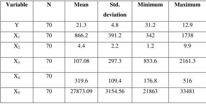
Table 1. Descriptive statistics
Variable N Mean Std.
deviation
Minimum Maximum
Y 70 21.3 4.8 31.2 12.9
X1 70 866.2 391.2 342 1738
X2 70 4.4 2.2 1.2 9.9
X3 70 107.08 297.3 853.6 2161.3
X4 70
319.6 109.4 176.8 516
X5 70 27873.09 3154.56 21863 33481
The table above shows the descriptive statistics of the variables of the model, in order to describe the nature of the variables under study. The following is an analytical presentation of these measures for each variable of the model. Mean unemployment rate in the sample was 21.3%, with the standard deviation 4.8%, while the lowest value is 31.2% and the highest value is 12.9%. The results also show that the mean value for the added value was 4429.9 million Iraqi dinars and a standard deviation 865.83 million Iraqi dinars. The mean inflation rate is 4.4%, while the lowest value was 1.2% and the highest value was 9.9 %. The results of the descriptive statistics show that the mean of the investment size is 1107.08 million Iraqi dinars and we noted also that the mean government expenditure was 319.6 million Iraqi dinars and a standard deviation was 109.4 million Iraqi dinars, while the lowest value of government expenditure was 176.8 million Iraqi dinars, and then highest value of government
expenditure is 516 million Iraqi dinars
.
Finally, the mean size of the population was 27873.0913
We started the analysis by running the K-M-O test to determine the sufficiency of the data. The K-O-M condition is that the minimum acceptable score is 0.5 for the sample size to be sufficient. The value of the K-M-O statistic is equal to 0.729, implying that the size of the sample used for the analysis is sufficient.
5.1. Detecting the multicollinearity problems
[image:14.595.192.407.384.542.2]The measures used for testing the existence of the multicollinearity in the model are, as previously described, CN and VIF. These indicators were computed for the regression parameters of all the explanatory variables of the model. The multicollinearity between the explanatory variables was revealed, as proven by the following results:
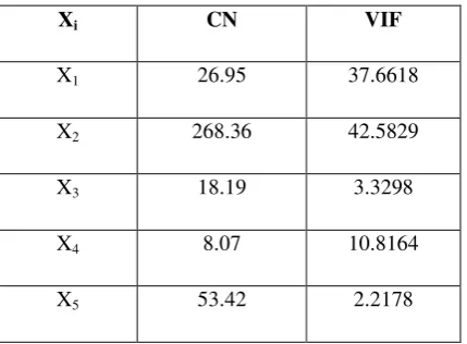
Table 2. Variance Inflation Factors and Condition Numbers
Xi CN VIF
X1 26.95 37.6618
X2 268.36 42.5829
X3 18.19 3.3298
X4 8.07 10.8164
X5 53.42 2.2178
We notice from Table 2 that the values of the VIF for some of the explanatory variables (X1, X2, X4) are greater than 10 and these variables suffer from inflation in the variance of their parameters: three variables are the cause of the multicollinearity problem. Also, as we note CN values of the explanatory variables X1, X2, X5 are greater than 20. This means that there is multicollinearity between these explanatory variables and in the following section the ridge regression method is used to address the multicollinearity issues.
5.2 Ridge regression analysis
14
multicollinearity between explanatory variables and the standard ridge regression coefficients were extracted for various values of the k parameter. The method of iterations (Hoerl, Kennard and Baldwin, 1976) was used to found the best value of the ridge parameter in accordance with formula (8). Using R package, we have run 50 iterations of this formula and reached the following:
𝑘 = 0.79857 .
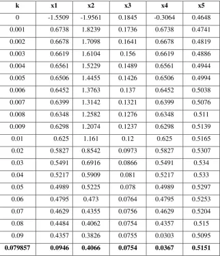
[image:15.595.137.460.316.691.2]In the next step, running the ridge regression models for various values of k ranging between 0.001 and 0.09, we have found the results presented in Table 3.
Table 3. Standardized ridge regression coefficients for various k values
k x1 x2 x3 x4 x5
0 -1.5509 -1.9561 0.1845 -0.3064 0.4648
0.001 0.6738 1.8239 0.1736 0.6738 0.4741
0.002 0.6678 1.7098 0.1641 0.6678 0.4819
0.003 0.6619 1.6104 0.156 0.6619 0.4886
0.004 0.6561 1.5229 0.1489 0.6561 0.4944
0.005 0.6506 1.4455 0.1426 0.6506 0.4994
0.006 0.6452 1.3763 0.137 0.6452 0.5038
0.007 0.6399 1.3142 0.1321 0.6399 0.5076
0.008 0.6348 1.2582 0.1276 0.6348 0.511
0.009 0.6298 1.2074 0.1237 0.6298 0.5139
0.01 0.625 1.161 0.12 0.625 0.5165
0.02 0.5827 0.8542 0.0973 0.5827 0.5307
0.03 0.5491 0.6916 0.0866 0.5491 0.534
0.04 0.5217 0.5909 0.081 0.5217 0.533
0.05 0.4989 0.5225 0.078 0.4989 0.5297
0.06 0.4795 0.473 0.0764 0.4795 0.5253
0.07 0.4629 0.4355 0.0756 0.4629 0.5204
0.08 0.4484 0.4062 0.0754 0.4357 0.515
0.09 0.4357 0.3826 0.0755 0.0303 0.5095
0.079857 0.0946 0.4066 0.0754 0.0367 0.5151
15
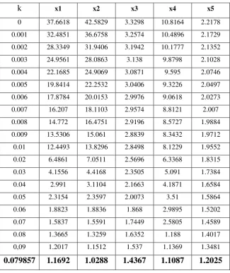
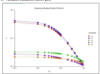
[image:16.595.135.461.167.555.2]The VIFs are computed for the all the previously standardized ridge regression models in order to test if the collinearity problem was solved and if the computed k is indeed the best value to be used in the final ridge regression model.
Table 4. Variance Inflation Factors
k x1 x2 x3 x4 x5
0 37.6618 42.5829 3.3298 10.8164 2.2178
0.001 32.4851 36.6758 3.2574 10.4896 2.1729
0.002 28.3349 31.9406 3.1942 10.1777 2.1352
0.003 24.9561 28.0863 3.138 9.8798 2.1028
0.004 22.1685 24.9069 3.0871 9.595 2.0746
0.005 19.8414 22.2532 3.0406 9.3226 2.0497
0.006 17.8784 20.0153 2.9976 9.0618 2.0273
0.007 16.207 18.1103 2.9574 8.8121 2.007
0.008 14.772 16.4751 2.9196 8.5727 1.9884
0.009 13.5306 15.061 2.8839 8.3432 1.9712
0.01 12.4493 13.8296 2.8498 8.1229 1.9552
0.02 6.4861 7.0511 2.5696 6.3368 1.8315
0.03 4.1556 4.4168 2.3505 5.091 1.7384
0.04 2.991 3.1104 2.1663 4.1871 1.6584
0.05 2.3154 2.3597 2.0073 3.51 1.5864
0.06 1.8823 1.8836 1.868 2.9895 1.5202
0.07 1.5837 1.5591 1.7449 2.5805 1.4589
0.08 1.3665 1.3259 1.6352 1.188 1.4017
0,09 1.2017 1.1512 1.537 1.1369 1.3481
0.079857 1.1692 1.0288 1.4367 1.1087 1.2025
The results from Table 4 show that in the particular case of k=0.079857, the levels of the VIFs for the explanatory variables are:
𝑉𝐼𝐹1 = 𝟏. 𝟏𝟔𝟗𝟐 , 𝑉𝐼𝐹2 = 𝟏. 𝟎𝟐𝟖𝟖 , VIF3 = 𝟏. 𝟒𝟑𝟔𝟕 , 𝐕𝐈𝐅𝟒 = 𝟏. 𝟏𝟎𝟖𝟕 , 𝐕𝐈𝐅𝟓 = 𝟏. 𝟐𝟎𝟐𝟓;
By simply comparing these with other values in the table, it seems that it is the best value to be selected, providing the lowest values for VIFs. (also see Figure 1 in Annex)
16
[image:17.595.72.548.157.402.2]regression model, using OLS for estimating the parameters. This comparison would help to better select the best model for dealing with multicollinearity in macroeconomic data.
Table 5. Ridge regression model vs. OLS: coefficients
Independent Variable
Coefficients Standard Errors
Regular Ridge
regression O.L.S.
Standardized Ridge regression
Standardized O.L.S.
Ridge
regression O.L.S.
Intercept 676.8475 -418.4163
x1 0.16892 -0.98586 0.0946 -1.5509 0.10825 0.47389
x2 0.05681 -0.31599 0.4066 -1.9561 0.02710 0.12805
x3 0.00443 0.01080 0.0754 0.1845 0.01090 0.01298
x4 0.06285 -0.02351 0.0367 -0.3064 0.01217 0.01561
X5 0.16014 0.02150 0.5151 0.4648 0.00797 0.00836
R-Squared 0.8723 0.9486
Sigma 481.6671 402.0432
It seems obvious that the values for standard errors in the ridge regression estimation method are better (and lower) than the values of standard errors when using the OLS estimation method; therefore, we conclude that ridge regression method reduces and could remove the multicollinearity problem between explanatory variables. The decision following this analysis is that the appropriate model for this study is:
𝑌 = 676.8475 + 0.16892X1+ 0.05681X2 + 0.00443 X3+ 0.062885 X4+ 0.16014 X5
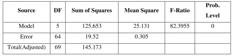
Table 6. Analysis of variance in the ridge regression model
Source DF Sum of Squares Mean Square F-Ratio Prob.
Level
Model 5 125.653 25.131 82.3955 0
Error 64 19.52 0.305
Total(Adjusted) 69 145.173
[image:17.595.103.493.622.716.2]17
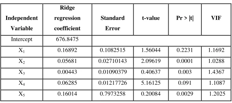
Table 7. Estimators of the ridge regression model
Independent Variable
Ridge regression coefficient
Standard Error
t-value Pr > |t| VIF
Intercept 676.8475
X1 0.16892 0.1082515 1.56044 0.2231 1.1692
X2 0.05681 0.02710143 2.09619 0.0001 1.0288
X3 0.00443 0.01090379 0.40637 0.003 1.4367
X4 0.06285 0.01217726 5.16125 0.091 1.1087
X5 0.16014 0.7973258 0.20084 0.0029 522221
The results presented in Table 7 show that the relationship between the unemployment rate in Iraq and the following three explanatory variables: inflation rate, volume of investment, size of the population is statistically significant, and the independent variables have a direct effect on unemployment. The relationship between the rate of inflation and the unemployment rate is positive, and the value of regression coefficient is 0.0568. This means that an increase in the inflation rate lead to an increase in the unemployment rate. The relationship between investments and the unemployment rate is also positive. The value of the regression coefficient is very low 0.00443, meaning that an increase in the volume of
investment could lead to a small increase in the unemployment rate. As for the relationship between the size of the population in the working-age group and unemployment rate, this is also positive. The value of the regression coefficient for this variable is 0.16014, meaning that
an increase in the size of the population will lead to an increase of the unemployment rate. These results are in line with our expectations, Iraq being a developing country, with a rigid labor market, affected more by external shocks than by internal development policies2 This also explains why the other two variables in the model have no significant effects on the unemployment rate.
6. Conclusions
18
was tested for identifying the factors that could explain the unemployment rate in an Arabic developing country, namely Iraq.
The study showed that the use of the ridge regression method in the cases when explanatory variables are affected by multicollinearity is one of the successful ways to solve this issue. Therefore, applying the ridge regression method in other studies is recommended, since it provides better estimators than the ordinary least square method when the explanatory variables are related, without omitting any of the explanatory variables.
By applying the ridge regression method, we found that there were three variables with a significant impact on the unemployment rate in Iraq: the rate of inflation, volume of investments and size of the population. Other variables (government expenditures or economic output) have a weak and non-statistical effect.The results are explained by the fact that the economic policies in Iraq are ineffective in reducing the unemployment rate, as the Iraqi economy is constantly exposed to various shocks, in both the supply and the demand.
References
Al-Hassan, Y. M. (2010). Performance of a new Ridge Regression Estimator. Journal of the Association of Arab Universities for Basic and Applied Sciences, 9(2), pp. 43-50.
Drapper, N.R. and Smith, H. (1981). Applied Regression Analysis, Second Edition,
New York: John Wiley and Sons.
El-Dereny, M. and Rashwan, N. (2011). Solving multicollinearity problem Using Ridge Regression Models. International Journal of Contemporary Mathematical. Sciences, 12, pp. 585 – 600.
Fitrianto, A. and Yik, L. C. (2014). Performance of Ridge Regression Estimator
Method on Small Sample size By Varying correlation coefficients: A simulation study. Journal of Mathematics and Statistics10 (1), pp. 25 – 29.
Hoerl, A. E.and R. W. Kennard. (1976). Ridge regression: iterative estimation of the
biasing parameter. Communication in Statist Theory and Method.5(1), pp. 77-88. Hoerl, A.E.and R.W. Kennard, Ridge Regression, 1980. Advances, Algorithms and
19
Hoerl, A.E., R.W. Kennard, and K.F. Baldwin. (1975). Ridge regression: some
simulations. Communications in Statistics- Theory and Methods, 4 (2), pp. 105-123.
Jaba, E., Balan, C.,Roman, M., Viorica, D. andRoman, M.(2008).Employment rate prognosis on the basis of the development environment trend displayed by years-clusters. Economic Computation and Economic Cybernetics Studies and Research
42(3-4), pp. 35-48.
Jaba, E.,Balan, C..Roman, M.andRoman, M.(2010).Statistical evaluation of
spatial concentration of unemployment by gender.Economic Computation and Economic Cybernetics Studies and Research, 44(3), pp. 79-92.
Kabbani, N. and Kothari, E. (2005). Youth employment in the MENA region: A
situational assessment. World Bank, Social Protection Discussion Paper, 534.
Kazem, A. H. and Muslim, B. H. (2002). Advanced Economic Measurement Theory and Practice. Baghdad: Duniaal-Amal Library.
Kibria, B.G. (2003). Performance of some new ridge regression estimators.
Communications in Statistics-Simulation and Computation,32 (2), pp. 419-435.
Massy, W. F. (1965). Principal Components Regression in Exploratory Statistical Research. Journal of the American Statistical Association,60(309), pp: 234-256.
Montgomery,D.C. and Peck, E. A. (1982). Introduction to linear regression analysis. New York: John Wiley and Sons.
Rencher, Alvin C., 2002. Method of Multivariate Analysis, New York: John Wiley& Sons.
Roman, M. (2003). Statistica financiar-bancar si bursiera. Bucuresti: Editura ASE
Shammari, M. H. (2013). Reality and causes of unemployment in Iraq after 2003.
Baghdad College of Economic Sciences Journal, 37, pp. 131-150.
Sifu, W. I., Chloff, F.H. and Jawad, S.I. (2006). Analytical Economical Problems, Prediction and Standard Tests of the Second Class. First Edition. Amman: Al Ahlia Press.
Willan, A.R. and Watts, D.G. (1978). Meaningful multicollinearity measures. Technometrics.20(4), p. 407-412.
Yong-wei, G., et al. (2008) A method to measure and test the damage of
20
[image:21.595.106.443.129.380.2]