732
Long Short-Term Memory
as a Dynamically Computed Element-wise Weighted Sum
Omer Levy∗ Kenton Lee∗ Nicholas FitzGerald Luke Zettlemoyer
Paul G. Allen School, University of Washington, Seattle, WA {omerlevy,kentonl,nfitz,lsz}@cs.washington.edu
Abstract
LSTMs were introduced to combat van-ishing gradients in simple RNNs by aug-menting them with gated additive recur-rent connections. We present an alterna-tive view to explain the success of LSTMs: the gates themselves are versatile recurrent models that provide more representational power than previously appreciated. We do this by decoupling the LSTM’s gates from the embedded simple RNN, produc-ing a new class of RNNs where the recur-rence computes an element-wise weighted sum of context-independent functions of the input. Ablations on a range of prob-lems demonstrate that the gating mecha-nism alone performs as well as an LSTM in most settings, strongly suggesting that the gates are doing much more in practice than just alleviating vanishing gradients.
1 Introduction
Long short-term memory (LSTM) (Hochreiter and Schmidhuber, 1997) has become the de-facto re-current neural network (RNN) for learning repsentations of sequences in NLP. Like simple re-current neural networks (S-RNNs) (Elman,1990), LSTMs are able to learn non-linear functions of arbitrary-length input sequences. However, they also introduce an additional memory cell to mit-igate the vanishing gradient problem (Hochreiter,
1991;Bengio et al.,1994). This memory is con-trolled by a mechanism of gates, whose additive connections allow long-distance dependencies to be learned more easily during backpropagation. While this view is mathematically accurate, in this paper we argue that it does not provide a complete picture of why LSTMs work in practice.
∗
The first two authors contributed equally to this paper.
We present an alternate view to explain the suc-cess of LSTMs: the gates themselves are power-ful recurrent models that provide more representa-tional power than previously realized. To demon-strate this, we first show that LSTMs can be seen as a combination of two recurrent models: (1) an S-RNN, and (2) an element-wise weighted sum of the S-RNN’s outputs over time, which is implicitly computed by the gates. We hypothesize that, for many practical NLP problems, the weighted sum serves as the main modeling component. The S-RNN, while theoretically expressive, is in practice only a minor contributor that clouds the mathemat-ical clarity of the model. By replacing the S-RNN with a context-independent function of the input, we arrive at a much more restricted class of RNNs, where the main recurrence is via the element-wise weighted sums that the gates are computing.
2 What Do Memory Cells Compute?
LSTMs are typically motivated as an augmenta-tion of simple RNNs (S-RNNs), defined as:
ht= tanh(Whhht−1+Whxxt+bh) (1)
S-RNNs suffer from the vanishing gradient prob-lem (Hochreiter,1991;Bengio et al.,1994) due to compounding multiplicative updates of the hidden state. By introducing a memory cell and an output layer controlled by gates, LSTMs enable shortcuts through which gradients can flow when learning with backpropagation. This mechanism enables learning of long-distance dependencies while pre-serving the expressive power of recurrent non-linear transformations provided by S-RNNs.
Rather than viewing the gates as simply an aux-iliary mechanism to address alearning problem, we present an alternate view that emphasizes their modeling strengths. We argue that the LSTM should be interpreted as a hybrid of two distinct recurrent architectures: (1) the S-RNN which pro-vides multiplicative connections across timesteps, and (2) the memory cell which provides additive connections across timesteps. On top of these re-currences, an output layer is included that simply squashes and filters the memory cell at each step.
Throughout this paper, let {x1, . . . ,xn}be the sequence of input vectors,{h1, . . . ,hn}be the se-quence of output vectors, and{c1, . . . ,cn}be the memory cell’s states. Then, given the basic LSTM definition below, we can formally identify three sub-components.
e
ct= tanh(Wchht−1+Wcxxt+bc) (2)
it=σ(Wihht−1+Wixxt+bi) (3)
ft=σ(Wf hht−1+Wf xxt+bf) (4)
ct=it◦cet+ft◦ct−1 (5)
ot=σ(Wohht−1+Woxxt+bo) (6)
ht=ot◦tanh(ct) (7)
Content Layer (Equation2) We refer toect as
the content layer, which is the output of an S-RNN. Evaluating the need for multiplicative recur-rent connections in the content layer is the focus of this work. The content layer is passed to the mem-ory cell, which decides which parts of it to store.
Memory Cell (Equations3-5) The memory cell
ct is controlled by two gates. The input gateit controls what part of the content (ect) is written
to the memory, while the forget gate ft controls
what part of the memory is deleted by filtering the previous state of the memory (ct−1). Writing to the memory is done by adding the filtered content (it◦ect) to the retained memory (ft◦ct−1).
Output Layer (Equations 6-7) The output layer ht passes the memory cell through a tanh activation function and uses an output gate ot to read selectively from the squashed memory cell.
Our goal is to study how much each of these components contribute to the empirical perfor-mance of LSTMs. In particular, it is worth consid-ering the memory cell in more detail to reveal why it could serve as a standalone powerful model of long-distance context. It is possible to show that it implicitly computes an element-wise weighted sumof all the previous content layers by expand-ing the recurrence relation in Equation5:
ct=it◦cet+ft◦ct−1
=
t
X
j=0
ij ◦ t
Y
k=j+1
fk
◦cej
=
t
X
j=0
wtj◦ecj
(8)
Each weightwtj is a product of the input gateij (when its respective inputcej was read) and every
subsequent forget gatefk. An interesting property of these weights is that, like the gates, they are also soft element-wise binary filters.
3 Standalone Memory Cells are Powerful
3.1 Simplified Models
The modeling power of LSTMs is commonly as-sumed to derive from the S-RNN in the content layer, with the rest of the model acting as a learn-ing aid to bypass the vanishlearn-ing gradient problem. We first isolate the S-RNN by ablating the gates (denoted asLSTM – GATESfor consistency).
To test whether the memory cell has enough modeling power of its own, we take an LSTM and replace the S-RNN in the content layer from Equation 2 with a simple linear transformation (cet=Wcxxt) creating theLSTM – S-RNNmodel.
We further simplify the LSTM by removing the output gate from Equation 7 (ht = tanh(ct)), leaving only the activation function in the output layer (LSTM – S-RNN – OUT). After removing the S-RNN and the output gate from the LSTM, the entire ablated model can be written in a modular, compact form:
ht=OUTPUT
Xt
j=0
wjt◦CONTENT(xj)
(9)
where the content layerCONTENT(·)and the out-put layerOUTPUT(·)are both context-independent functions, making the entire model highly con-strained and mathematically simpler. The com-plexity of modeling contextual information is needed only for computing the weights wtj. As we will see in Section3.2, both of these ablations perform on par with LSTMs on several tasks.
Finally, we ablate the hidden state from the gates as well, by computing each gate gt via σ(Wgxxt+bg). In this model, the only recurrence is the additive connection in the memory cell; it has no multiplicative recurrent connections at all. It can be seen as a type of QRNN (Bradbury et al.,
2016) or SRU (Lei et al.,2017b), but for consis-tency we label it asLSTM – S-RNN – HIDDEN.
3.2 Experiments
We compare model performance on four NLP tasks, with an experimental setup that is lenient towards LSTMs and harsh towards its simplifica-tions. In each case, we use existing implementa-tions and previously reported hyperparameter set-tings. Since these settings were tuned for LSTMs, any simplification that performs equally to (or bet-ter than) LSTMs under these LSTM-friendly set-tings provides strong evidence that the ablated component is not a contributing factor. For each
task we also report the mean and standard devia-tion of 5 runs of the LSTM settings to demonstrate the typical variance observed due to training with different random initializations.
Language Modeling We evaluate the models on the Penn Treebank (PTB) (Marcus et al., 1993) language modeling benchmark. We use the im-plementation of Zaremba et al.(2014) from Ten-sorFlow’s tutorial while replacing any invocation of LSTMs with simpler models. We test two of their configurations:mediumandlarge(Table1).
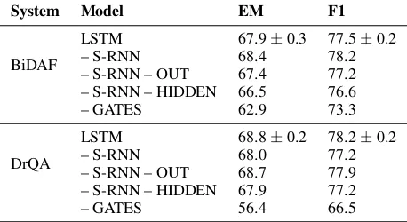
Question Answering For question answering, we use two different QA systems on the Stan-ford question answering dataset (SQuAD) ( Ra-jpurkar et al., 2016): the Bidirectional Atten-tion Flow model (BiDAF) (Seo et al., 2016) and DrQA (Chen et al., 2017). BiDAF contains 3 LSTMs, which are referred to as the phrase layer, the modeling layer, and the span end en-coder. Our experiments replace each of these LSTMs with their simplified counterparts. We di-rectly use the implementation of BiDAF from Al-lenNLP (Gardner et al.,2017), and all experiments reuse the existing hyperparameters that were tuned for LSTMs. Likewise, we use an open-source implementation of DrQA1 and replace only the LSTMs, while leaving everything else intact. Ta-ble2shows the results.
Dependency Parsing For dependency pars-ing, we use the Deep Biaffine Dependency Parser (Dozat and Manning, 2016), which relies on stacked bidirectional LSTMs to learn context-sensitive word embeddings for determining arcs between a pair of words. We directly use their re-leased implementation, which is evaluated on the Universal Dependencies English Web Treebank v1.3 (Silveira et al., 2014). In our experiments, we use the existing hyperparameters and only re-place the LSTMs with the simplified architectures. Table3shows the results.
Machine Translation For machine translation, we used OpenNMT (Klein et al.,2017) to train En-glish to German translation models on the multi-modal benchmarks from WMT 2016 (used in OpenNMT’s readme file). We use OpenNMT’s default model and hyperparameters, replacing the stacked bidirectional LSTM encoder with the
Configuration Model Perplexity
PTB (Medium)
LSTM 83.9±0.3
– S-RNN 80.5
– S-RNN – OUT 81.6
– S-RNN – HIDDEN 83.3
– GATES 140.9
PTB (Large)
LSTM 78.8±0.2
– S-RNN 76.0
– S-RNN – OUT 78.5
– S-RNN – HIDDEN 82.9
[image:4.595.311.518.64.134.2]– GATES 126.1
Table 1: Performance on language modeling benchmarks, measured by perplexity.
System Model EM F1
BiDAF
LSTM 67.9±0.3 77.5±0.2
– S-RNN 68.4 78.2
– S-RNN – OUT 67.4 77.2
– S-RNN – HIDDEN 66.5 76.6
– GATES 62.9 73.3
DrQA
LSTM 68.8±0.2 78.2±0.2
– S-RNN 68.0 77.2
– S-RNN – OUT 68.7 77.9
– S-RNN – HIDDEN 67.9 77.2
– GATES 56.4 66.5
Table 2: Performance on SQuAD, measured by exact match (EM) and span overlap (F1).
plified architectures.2Table4shows the results.
3.3 Discussion
We showed four major ablations of the LSTM. In the S-RNN experiments (LSTM – GATES), we ab-late the memory cell and the output layer. In the LSTM – S-RNNandLSTM – S-RNN – OUT exper-iments, we ablate the S-RNN. In the LSTM – S-RNN – HIDDEN, we remove not only the S-S-RNN in the content layer, but also the S-RNNs in the gates, resulting in a model whose sole recurrence is in the memory cell’s additive connection.
As consistent with previous literature, removing the memory cell degrades performance drastically. In contrast, removing the S-RNN makes little to no difference in the final performance, suggesting that the memory cell alone is largely responsible for the success of LSTMs in NLP.
Even after removing every multiplicative recur-rence from the memory cell itself, the model’s performance remains well above the vanilla
S-2For the S-RNN baseline (
LSTM – GATES), we had to tune the learning rate to 0.1 because the default value (1.0) resulted in exploding gradients. This is the only case where hyperparameters were modified in all of our experiments.
Model UAS LAS
LSTM 90.60±0.21 88.05±0.33
– S-RNN 90.77 88.49
– S-RNN – OUT 90.70 88.31
– S-RNN – HIDDEN 90.53 87.96
[image:4.595.341.488.195.268.2]– GATES 87.75 84.61
Table 3: Performance on the universal dependen-cies parsing benchmark, measured by unlabeled (UAS) and labeled attachment score (LAS).
Model BLEU
LSTM 38.19±0.1
– S-RNN 37.84
– S-RNN – OUT 38.36 – S-RNN – HIDDEN 36.98
– GATES 26.52
Table 4: Performance on the WMT 2016 multi-modal English to German benchmark.
RNN’s, and falls within the standard deviation of an LSTM’s on some tasks (see Table3). This latter result indicates that the additive recurrent connec-tion in the memory cell – and not the multiplicative recurrent connections in the content layer or in the gates – is the most important computational ele-ment in an LSTM. As a corollary, this result also suggests that a weighted sum of context words, while mathematically simple, is a powerful model of contextual information.
4 LSTM as Self-Attention
Attention mechanisms are widely used in the NLP literature to aggregate over a sequence (Cho et al.,
2014;Bahdanau et al.,2015) or contextualize to-kens within a sequence (Cheng et al.,2016;Parikh et al., 2016) by explicitly computing weighted sums. In the previous sections, we demonstrated that LSTMs implicitly compute weighted sums as well, and that this computation is central to their success. How, then, are these two computations related, and in what ways do they differ?
[image:4.595.72.301.239.364.2]simplified LSTM’s weights as is commonly done with attention (see AppendixAfor visualization). However, there are three major differences in how theweightswtjare computed.
First, the LSTM’s weights are vectors, while attention typically computes scalar weights; i.e. a separate weighted sum is computed for every dimension of the LSTM’s memory cell. Multi-headed self-attention (Vaswani et al., 2017) can be seen as a middle ground between the two ap-proaches, allocating a scalar weight for different subsets of the dimensions.
Second, the weighted sum is accumulated with a dynamic program. This enables a linear rather than quadratic complexity in comparison to self-attention, but reduces the amount of parallel com-putation. This accumulation also creates an induc-tive bias of attending to nearby words, since the weights can only decrease over time.
Finally, attention has a probabilistic interpreta-tion due to the softmax normalizainterpreta-tion, while the sum of weights in LSTMs can grow up to the se-quence length. In variants of the LSTM that tie the input and forget gate, such as coupled-gate LSTMs (Greff et al., 2016) and GRUs (Cho et al.,2014), the memory cell instead computes a weighted av-erage with a probabilistic interpretation. These variants compute locally normalized distributions via a product of sigmoids rather than globally nor-malized distributions via a single softmax.
5 Related Work
Many variants of LSTMs (Hochreiter and Schmid-huber, 1997) have been previously explored. These typically consist of a different parameteri-zation of the gates, such as LSTMs with peephole connections (Gers and Schmidhuber,2000), or a rewiring of the connections, such as GRUs (Cho et al.,2014). However, these modifications invari-ably maintain the recurrent content layer. Even more systematic explorations (J´ozefowicz et al.,
2015;Greff et al., 2016;Zoph and Le, 2017) do not question the importance of the embedded S-RNN. This is the first study to provide apples-to-apples comparisons between LSTMs with and without the recurrent content layer.
Several other recent works have also reported promising results with recurrent models that are vastly simpler than LSTMs, such as quasi-recurrent neural networks (Bradbury et al.,2016), strongly-typed recurrent neural networks (
Bal-duzzi and Ghifary, 2016), recurrent additive net-works (Lee et al., 2017), kernel neural net-works (Lei et al., 2017a), and simple recurrent units (Lei et al.,2017b), making it increasingly ap-parent that LSTMs are over-parameterized. While these works indicate an obvious trend, they do not focus on explaining what LSTMs are learning. In our carefully controlled ablation studies, we pro-pose and evaluate the minimal changes required to test our hypothesis that LSTMs are powerful because they dynamically compute element-wise weighted sums of content layers.
6 Conclusion
We presented an alternate view of LSTMs: they are a hybrid of S-RNNs and a gated model that dy-namically computes weighted sums of the S-RNN outputs. Our experiments investigated whether the S-RNN is a necessary component of LSTMs. In other words, are the gates alone as powerful of a model as an LSTM? Results across four ma-jor NLP tasks (language modeling, question an-swering, dependency parsing, and machine trans-lation) indicate that LSTMs suffer little to no per-formance loss when removing the S-RNN. This provides evidence that the gating mechanism is doing the heavy lifting in modeling context. We further ablate the recurrence in each gate and find that this incurs only a modest drop in performance, indicating that the real modeling power of LSTMs stems from their ability to compute element-wise weighted sums of context-independent functions of their inputs.
This realization allows us to mathemati-cally relate LSTMs and other gated RNNs to attention-based models. Casting an LSTM as a dynamically-computed attention mechanism en-ables the visualization of how context is used at every timestep, shedding light on the inner work-ings of the relatively opaque LSTM.
Acknowledgements
References
Yossi Adi, Einat Kermany, Yonatan Belinkov, Ofer Lavi, and Yoav Goldberg. 2017. Fine-grained anal-ysis of sentence embeddings using auxiliary predic-tion tasks. InICLR.
Dzmitry Bahdanau, Kyunghyun Cho, and Yoshua
Ben-gio. 2015. Neural machine translation by jointly
learning to align and translate. InICLR.
David Balduzzi and Muhammad Ghifary. 2016.
Strongly-typed recurrent neural networks. In Pro-ceedings of the 33nd International Conference on Machine Learning, ICML 2016, New York City, NY, USA, June 19-24, 2016. pages 1292–
1300. http://jmlr.org/proceedings/
papers/v48/balduzzi16.html.
Yoshua Bengio, Patrice Y. Simard, and Paolo Frasconi. 1994. Learning long-term dependencies with gradi-ent descgradi-ent is difficult. IEEE Transactions on Neu-ral Networks5(2):157–166.
James Bradbury, Stephen Merity, Caiming Xiong, and Richard Socher. 2016. Quasi-recurrent neural
net-works. CoRRabs/1611.01576.
Danqi Chen, Adam Fisch, Jason Weston, and
An-toine Bordes. 2017. Reading wikipedia to answer
open-domain questions. InProceedings of the 55th Annual Meeting of the Association for Computa-tional Linguistics (Volume 1: Long Papers). Asso-ciation for Computational Linguistics, Vancouver,
Canada, pages 1870–1879. http://aclweb.
org/anthology/P17-1171.
Jianpeng Cheng, Li Dong, and Mirella Lapata. 2016.
Long short-term memory-networks for machine reading. In Proceedings of the 2016 Conference on Empirical Methods in Natural Language Pro-cessing. Association for Computational
Linguis-tics, Austin, Texas, pages 551–561. https://
aclweb.org/anthology/D16-1053.
Kyunghyun Cho, Bart van Merrienboer, Caglar Gul-cehre, Dzmitry Bahdanau, Fethi Bougares, Holger
Schwenk, and Yoshua Bengio. 2014. Learning
phrase representations using rnn encoder–decoder for statistical machine translation. InProceedings of the 2014 Conference on Empirical Methods in Natural Language Processing (EMNLP). Associa-tion for ComputaAssocia-tional Linguistics, Doha, Qatar,
pages 1724–1734. http://www.aclweb.org/
anthology/D14-1179.
Timothy Dozat and Christopher D. Manning. 2016. Deep biaffine attention for neural dependency
pars-ing. CoRRabs/1611.01734.
Jeffrey L. Elman. 1990. Finding structure in time.
Cognitive Science14:179–211.
Matt Gardner, Joel Grus, Mark Neumann, Oyvind Tafjord, Pradeep Dasigi, Nelson Liu, Matthew Pe-ters, Michael Schmitz, and Luke Zettlemoyer. 2017.
Allennlp: A deep semantic natural language pro-cessing platform. http://allennlp.org/ papers/AllenNLP_white_paper.pdf.
Felix A. Gers and J¨urgen Schmidhuber. 2000. Recur-rent nets that time and count. InIJCNN.
Klaus Greff, Rupesh K Srivastava, Jan Koutn´ık, Bas R Steunebrink, and J¨urgen Schmidhuber. 2016. Lstm:
A search space odyssey.IEEE Transactions on
Neu-ral Networks and Learning Systems.
Luheng He, Kenton Lee, Mike Lewis, and Luke Zettle-moyer. 2017. Deep semantic role labeling: What
works and whats next. In Proceedings of the
An-nual Meeting of the Association for Computational Linguistics.
Sepp Hochreiter. 1991. Untersuchungen zu
dynamis-chen neuronalen netzen. Diploma, Technische
Uni-versit¨at M¨unchen91.
Sepp Hochreiter and J¨urgen Schmidhuber. 1997.
Long Short-term Memory. Neural computation
9(8):1735–1780.
Rafal J´ozefowicz, Wojciech Zaremba, and Ilya
Sutskever. 2015. An empirical exploration of recur-rent network architectures. InICML.
Guillaume Klein, Yoon Kim, Yuntian Deng, Jean
Senellart, and Alexander M. Rush. 2017. Opennmt:
Open-source toolkit for neural machine translation. InProc. ACL.https://doi.org/10.18653/ v1/P17-4012.
Kenton Lee, Omer Levy, and Luke Zettlemoyer.
2017. Recurrent additive networks. arXiv preprint
arXiv:1705.07393.
Tao Lei, Wengong Jin, Regina Barzilay, and Tommi Jaakkola. 2017a. Deriving neural architectures from
sequence and graph kernels. InICML.
Tao Lei, Yu Zhang, and Yoav Artzi. 2017b.
Train-ing rnns as fast as cnns. arXiv preprint
arXiv:1709.02755.
Tal Linzen, Emmanuel Dupoux, and Yoav Goldberg. 2016. Assessing the ability of lstms to learn
syntax-sensitive dependencies.TACL4:521–535.
Mitchell P. Marcus, Beatrice Santorini, and Mary Ann Marcinkiewicz. 1993. Building a large annotated
corpus of english: The penn treebank.
Computa-tional Linguistics19:313–330.
Ankur Parikh, Oscar T¨ackstr¨om, Dipanjan Das, and
Jakob Uszkoreit. 2016. A decomposable
atten-tion model for natural language inference. In
Proceedings of the 2016 Conference on Empiri-cal Methods in Natural Language Processing. As-sociation for Computational Linguistics, Austin,
Texas, pages 2249–2255. https://aclweb.
Pranav Rajpurkar, Jian Zhang, Konstantin Lopyrev, and Percy Liang. 2016. Squad: 100, 000+ questions for
machine comprehension of text. InEMNLP.
Min Joon Seo, Aniruddha Kembhavi, Ali Farhadi,
and Hannaneh Hajishirzi. 2016. Bidirectional
at-tention flow for machine comprehension. CoRR
abs/1611.01603.
Natalia Silveira, Timothy Dozat, Marie-Catherine de Marneffe, Samuel Bowman, Miriam Connor, John Bauer, and Christopher D. Manning. 2014. A gold standard dependency corpus for English. In
Proceedings of the Ninth International Conference on Language Resources and Evaluation (LREC-2014).
Ashish Vaswani, Noam Shazeer, Niki Parmar, Jakob Uszkoreit, Llion Jones, Aidan N. Gomez, Lukasz Kaiser, and Illia Polosukhin. 2017. Attention is all
you need. arXiv preprint arXiv:1706.03762.
Wojciech Zaremba, Ilya Sutskever, and Oriol Vinyals.
2014. Recurrent neural network regularization.
arXiv preprint arXiv:1409.2329.
Barret Zoph and Quoc V Le. 2017. Neural architecture search with reinforcement learning. InICLR.
A Weight Visualization
Given the empirical evidence that LSTMs are ef-fectively learning weighted sums of the content layers, it is natural to investigate what weights the model learns in practice. Using the more mathe-matically transparent simplification of LSTMs, we can visualize the weightswjtthat are placed on ev-ery inputjat every timestept(see Equation 9).
Unlike attention mechanisms, these weights are vectors rather than scalar values. Therefore, we can only provide a coarse-grained visualization of the weights by rendering theirL2-norm, as shown in Table 5. In the visualization, each column indicates the word represented by the weighted sum, and each row indicates the word over which the weighted sum is computed. Dark horizontal streaks indicate the duration for which a word was remembered. Unsurprisingly, the weights on the diagonal are always the largest since it indicates the weight of the current word. More interesting task-specific patterns emerge when inspecting the off-diagonals that represent the weight on the con-text words.
The first visualization uses the language model. Due to the language modeling setup, there are only non-zero weights on the current or previous words. We find that the common function words are quickly forgotten, while infrequent words that
signal the topic are remembered over very long distances.
The second visualization uses the dependency parser. In this setting, since the recurrent architec-tures are bidirectional, there are non-zero weights on all words in the sentence. The top-right triangle indicates weights from the forward direction, and the bottom-left triangle indicates from the back-ward direction. For syntax, we see a significantly different pattern. Function words that are useful for determining syntax are more likely to be re-membered. Weights on head words are also likely to persist until the end of a constituent.
739
Language model weights Dependency parser weights
The hymn was sung at my first inauguralchurchserviceas governor
The hymn was sung at my first inaugural church service as governor
The hymn was sung at my first inauguralchurchserviceas governor
The hymn was sung at my first inaugural church service as governor
US troopsthere clashedwith guerrillasin a fight that left one Iraqi dead
US troops there clashed with guerrillas in a fight that left one Iraqi dead
US troopsthere clashedwith guerrillasin a fight that left one Iraqi dead
US troops there clashed with guerrillas in a fight that left one Iraqi dead
He did commenton what he meant by the phrase .
He did comment on what he meant by the phrase .
He did commenton what he meant by the phrase .
He did comment on what he meant by the phrase .
I spoke to Bruce Garcey at NiMo regardingtheir RFP
I spoke to Bruce Garcey at NiMo regarding their RFP
I spoke to Bruce Garcey at NiMo regardingtheir RFP
I spoke to Bruce Garcey at NiMo regarding their RFP