An econometric evaluation of daylight saving time in Mexico

Munich Personal RePEc Archive

An econometric evaluation of daylight

saving time in Mexico

Flores, Daniel and Luna, Edgar

Universidad Autónoma de Nuevo León, Universidad Autónoma de

Nuevo León

2018

Online at

https://mpra.ub.uni-muenchen.de/89678/

1

An econometric evaluation of daylight saving time in Mexico

Daniel Flores

Edgar M. Luna

Facultad de Economía, Universidad Autónoma de Nuevo León

Unidad Mederos, Ave. Lázaro Cárdenas 4600 Oriente, Monterrey, N.L., 64930, MEXICO

Abstract

This paper evaluates the impact of daylight saving time (DST) on households’ consumption of electricity in Mexico. Differences-in-differences estimates suggest that current savings in households’ electricity consumption due to DST account for almost 0.6% of total electricity consumption in the country. Nevertheless, the effect of DST is not homogeneous along the whole period in which it is in effect (from April to October). Savings are larger toward the end of the period.

Keywords: Daylight saving time; time series, Mexico

JEL Classification codes: Q48

1. Introduction

Daylight saving time (DST) is a common practice in several countries around the world.

Although Benjamin Franklin is acknowledged as the promoter of the idea at the end of the 18th

century, it was actually implemented by some countries in Europe and the United States (US)

until the First World War. Since then, several countries have been using it intermittently.

According to the information in the web page of Fideicomiso para el Ahorro de Energia Electrica

(FIDE),1 _{DST is currently used in 86 countries around the world. Among other things, this is due}

to the idea that it saves energy and, consequently, reduces the use of natural resources.

DST is supposed to generate two main types of savings (Maqueda and Rebolledo, 2008).

On the one hand, it changes the consumption pattern in households by reducing electricity

consumption in the evening, during the peak of demand, and increasing it early in the morning

(Kellogg and Wolff, 2008). Hence, DST helps to smooth consumption during the day generating

efficiency gains in the production of electricity. On the other hand, DST is assumed to reduce

1 _{FIDE is a trust fund created by the Mexican government to promote savings in electricity usage.}

2

overall electricity consumption. That is, reduced consumption during the evening –attributed to

DST– is larger than increased consumption during the morning.

There are some recent studies arguing that DST, or an extension of its duration, does not

necessarily generate energy savings. For example, the works of Kellogg and Wolff (2008),

Kotchen and Grant (2011), and Marshall (2010), based on natural experiments in Australia, the

US, and Chile, respectively, claim that implementing DST or extending its duration actually

increases overall electricity consumption. Similarly, Shimoda et al. (2007), using simulation

techniques, find that DST would increase residential electricity consumption in Osaka; while

Kandel and Sheridan (2007), using a time series approach, find that DST has an ambiguous

effect on electricity consumption in California. However, many other recent studies find the

opposite (Maqueda and Rebolledo, 2008; Mirza and Bergland, 2011; Ahuja and SenGupta, 2012;

Verdejo et al., 2016).

Mexico is an interesting place to evaluate DST for several reasons. First, while the US

and other developed countries have a long experience using DST, Mexico has been using it only

for a few years.2 _{Therefore, there is recent and reliable information on household consumption}

both before and after DST was implemented. Second, the DST is used only during part of the

year. In particular, individuals in Mexico adjust their clocks one hour forward the first Sunday of

April and adjust them backward the last Sunday of October. Hence, some months of the year

(those not affected by DST) can be used as a control group in order to evaluate DST using a

differences-in-differences (DD) approach. Third, the price of electricity for household

consumption in Mexico is regulated (fixed by the government). Therefore, price is not an

endogenous variable in Mexico as it is in other places.3 _{Fourth, the most recent evaluation of}

DST in Mexico –conducted by Maqueda and Rebolledo (2008)– took place about 10 years ago.

In this paper, we evaluate empirically whether DST reduces or not overall household

electricity consumption in Mexico. Moreover, we evaluate the effect of DST for each of the

months included in the program. Our results, based on publicly available data gathered from the

2 _{Choi, Pellen and Masson (2017) make a similar argument to motivate their study about the effects of DST in}

Western Australia (WA). They explain that DST was adopted in WA at the end of 2006 and then repealed at the beginning of 2009.

3 _{Mexico is not the only country in which electricity prices are fixed by the government. For instance, Kellogg and}

3

national statistics agency in Mexico (INEGI), indicate that DST reduces consumption. We

estimate that household electricity consumption savings generated by DST are about 1,545

Gigawatts/hour (GWh) on a yearly basis. These savings account for almost 0.6% of total

electricity consumption in the country. Nevertheless, DST does not reduce consumption

uniformly during the whole period. In particular, we find that DST has smaller effects during the

first months of the period (that is, April, May, June and July) and larger effects towards the last

months (that is, August, September, and October).

The rest of the paper is organized as follows. In Section 2, we explain the basic

characteristics of the Mexican electricity industry. In Section 3, we make simple DD calculations

around the point in which DST was implemented for the first time in order to have a first

approximation of the impact of this policy. In Section 4, we estimate the effects of DST

econometrically. In Section 5, we conduct robustness tests. Finally, in the last section, we present

the main conclusions if this study.

2. Background

The electricity industry has been subject to several regulatory changes in Mexico. These

changes point slowly towards the creation of a private wholesale market for electricity. For many

years, the state-owned public utility Comisión Federal de Electricidad (CFE) was by law the

unique producer and distributor of electricity in the country. At the beginning of the 90s, there

was a change in the law allowing private firms to generate electricity for own-consumption or to

sell it to CFE. The most recent reform –approved in the year 2013– allowed private firms to

generate and distribute electricity in the country.

In spite of creating a wholesale electricity market in Mexico, the recent energy reform

maintained CFE as a monopoly in the distribution of electricity for household consumption.

Moreover, the prices of electricity for households are still fixed by the Ministry of Finance

(SHCP), taking into account the opinion of other ministries as well as CFE proposals. It follows

that these prices are not driven by market conditions, but by an authority that takes into account

economic, social, and political issues.

Electricity prices for households vary with the season, the geographical region of the

4

Prices are lower during the summer semester when temperatures are relatively high in most of

the country. In addition, prices vary from region to region depending on historical temperature

records. Prices are lower in the regions where the average minimum temperature has been higher

in the last years. The idea behind this pricing policy is to compensate households that face

warmer summers and, consequently, need to spend more on air conditioning (AC). Finally,

households face an increasing block tariff. That is, the marginal price of electricity increases

when consumption reaches certain thresholds. This pricing policy is intended to have the

following effects. On the one hand, it charges higher prices at the margin to higher income

households because they tend to consume more electricity. On the other hand, it promotes energy

savings.

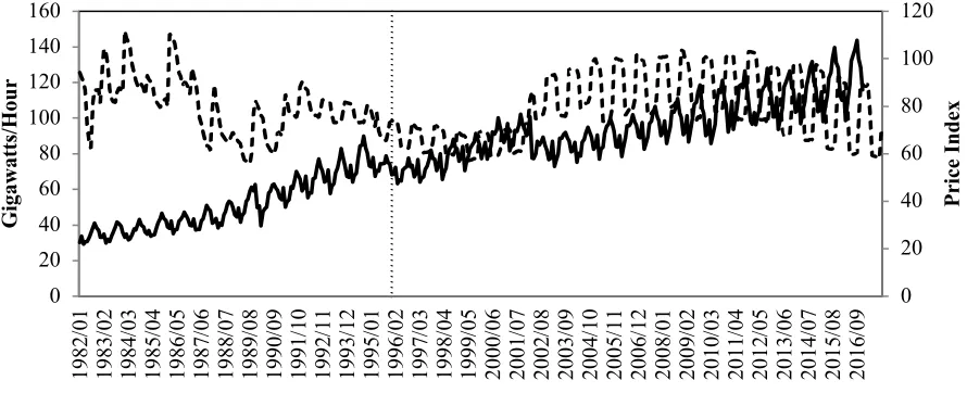
Fig. 1. Daily domestic consumption and real prices of electricity in Mexico. Data source: www.inegi.org.mx

Figure 1 illustrates the evolution of the monthly average of households’ daily electricity

consumption in Mexico and its real average price. Consumption is measured in GWh, while the

real price of electricity is an index of domestic electricity prices divided by the national

consumer price index. Electricity consumption exhibits a clear increasing trend over the whole

period. In contrast, the real price of electricity has been relatively stable if we ignore seasonal

variations. This occurs because the SHCP adjusts prices periodically to keep up with the inflation

rate. However, there are several subtle but clear shifts in the price trend. That is, electricity prices 0 20 40 60 80 100 120 0 20 40 60 80 100 120 140 160 1982 /01 1983 /02 1984 /03 1985 /04 1986 /05 1987 /06 1988 /07 1989 /08 1990 /09 1991 /10 1992 /11 1993 /12 1995 /01 1996 /02 1997 /03 1998 /04 1999 /05 2000 /06 2001 /07 2002 /08 2003 /09 2004 /10 2005 /11 2006 /12 2008 /01 2009 /02 2010 /03 2011 /04 2012 /05 2013 /06 2014 /07 2015 /08 2016 /09 Pr ic e Inde x Gi g a w a tt s/ Ho u r

5

tended to fall during the 90s, to increase at the beginning of the next decade, and to fall again at

the beginning of the last decade. Now, if we consider seasonal variations in consumption, it is

easy to note that peaks take place during the summer mainly for two reasons: need for AC and

low electricity prices.

The thin vertical dotted line in Figure 1 divides the timeline into two parts: before and

after the implementation of DST in the country. The Mexican government started implementing

DST in 1996, while prices and consumption of electricity were moving mainly due to seasonal

adjustments. In addition, the country suffered a deep economic crisis in the middle of the 90s, a

small one at the beginning of the next decade, and a large one again after the 2008 World

Financial Crisis. It follows that it is not straightforward to separate the effect of DST on

electricity consumption from that of other variables.

3. Differences-in-differences comparisons

In this section, we make simple differences-in-differences (DD) comparisons to have an

initial approximation of the impact of DST on domestic consumption of electricity. It is

important to explain that we will evaluate the effect of DST econometrically in the next section.

At this point, we will simply compare domestic consumption during different months of the year

before and after the implementation of DST for illustration purposes. Given that DST started in

1996, we compare average consumption in years 1993, 1994 and 1995 with the average in years

1996, 1997 and 1998. Similarly, given that DST takes place only during part of the year, we use

months to build control and treatment groups. The control group includes the months of January,

February, March, November and December, while the treatment group includes the remaining 7

months. That is, the treatment group includes only the months where DST is applied.

The idea of using months as controls to estimate the effect of DST is not new. Kellogg

and Wolff (2008) tried using months adjacent to DST in Australia (that is, August and

November) as controls. However, they decided not to rely on the estimates they obtained using

this approach because monthly demand in Australia is not stable. We try to avoid this problem, at

least partially, by using a three-year average of monthly consumption for these comparisons.

non-6

DST months in a given year as controls. Again, this idea is not completely new. Choi, Pellen and

Masson (2017) use non-DST months as controls in their econometric analysis.

We believe that using months to construct the treatment and control groups is appropriate

for several reasons. First, the choice of months where DST applies is arbitrary to some extent. It

is clear that DST generates more savings in the summer than during the rest of the year.

However, some countries have discussed and implemented year round DST or extensions of

DST.4 _{Second, households’ electricity consumption seemed to be growing homogenously around}

those years. Third, this approach produces a reasonable and simple first approximation to the

effects of DST on electricity consumption.

Table 1. Average household electricity consumption in Mexico (GWh) Before After Change % Change DST January 2,111.33 2,179.33 68.00 3.22 No February 2,073.33 2,160.33 87.00 4.20 No

March 1,956.00 1,992.67 36.67 1.87 No

April 2,001.67 2,006.33 4.67 0.23 Yes

May 2,093.33 2,107.67 14.33 0.68 Yes

June 2,200.67 2,212.00 11.33 0.51 Yes

July 2,382.00 2,357.33 -24.67 -1.04 Yes August 2,452.00 2,421.67 -30.33 -1.24 Yes September 2,517.00 2,473.67 -43.33 -1.72 Yes October 2,435.00 2,411.00 -24.00 -0.99 Yes November 2,283.33 2,332.00 48.67 2.13 No December 2,159.00 2,204.67 45.67 2.12 No

Average Average Difference % Non DST months 2,116.60 2,173.80 57.20 2.70

DST months 2,297.38 2,284.24 -13.14 -0.57

Differences-in-differences 70.34 3.27

Table 1 suggests that DST was effective to reduce domestic electricity consumption in

Mexico, or at least to make it grow at a slower rate. The first two columns of data in the table are

three-year averages of domestic consumption before and after, respectively, the implementation

of DST. The third column in the table is the percentage change when comparing average

consumption before and after DST for a given month. The last column specifies whether DST

applies or not in the corresponding month. Note that consumption increases between 1.87% and

4 _{See HMSO (1970), Ebersale et al. (1974), Kellogg and Wolff (2008), Hill et al. (2010), and Ahuja and SenGupta}

7

4.2% in the months that belong to the control group (that is, the five months in which DST is not

implemented in Mexico). In contrast, consumption decreases (or increases a little bit) in the

months that belong to the treatment group.

In order to calculate an overall DD estimate of the effect of DST, we compare the rates of

growth of the treatment and control groups. In this case, the growth of average domestic

consumption in DST months is -0.57% while its counterpart is 2.7%. This simple DD

comparison suggests then that DST reduced average domestic consumption about 70 GWh

monthly. If this number is correct, the DST allowed saving about 490 GWh per year. Total

electricity use in Mexico, at that time, was about 135 thousand GWh. Therefore, savings

represented about 0.36% of total electricity consumption in the country when DST was

implemented for the first time. This number is clearly lower than previous estimates. For

instance, Ramos et al. (1998) calculated that DST reduced total electricity use in Mexico

between 0.65% and 1.1%.

4. Econometric estimate of the effect of DST

In this section, we use monthly time series data to estimate econometrically the effect of

DST on household electricity consumption.5 _{The database covers the period from 1982 to 2016}

and is published by INEGI. The main variable of interest in our study is average (daily)

households’ consumption of electricity during the month.6 _{We choose to use household}

consumption data because most savings from DST are expected to take place in households’

electricity consumption for illumination (Aries and Newsham, 2008; Momani, Yatim and Ali,

2009).

Assume that daily average household consumption of electricity (Q) during month of

year is given by the following expression:

(1) .

5 _{CFE classifies consumers in three types: residential, commercial and industrial. Household consumption}

corresponds to consumers classified as residential.

6 _{We consider April and October as part of treatment months because more than 75% of the days in the month are}

DST days.

i

t

it it i

t it

it PR Y W DST

8

The variables that explain household consumption of electricity are: real price of electricity (PR),

households’ permanent income (Y) during the year, weather conditions (W) during the month,

whether DST is in effect or not, and an error term.

We will use the sub-index letter o to denote that a variable belongs to the control group

(that is, a month or set of months in which DST is not implemented). Therefore, we can calculate

the difference between consumption in a given treatment month and the control period as

follows

(2) .

Variables that adjust every year like households’ permanent income (Y) disappear once

we calculate differences in household consumption of energy. Similarly, seasonal differences

(such as daylight hours or weather conditions) between a particular month and the control

month(s) become a constant. We can rewrite (2) in terms of percentage changes as follows

(3) .

We can define as the difference between average daily

consumption during month and the month or set of months used as controls. Similarly, we can

also define . Finally, we can simplify (3) to obtain

(4) .

We estimate this equation pooling together all the months in which DST is implemented.

Note that is zero from years 1982 to 1995 and one afterwards. It is reasonable to argue

that differences in weather conditions between summer and winter months have been changing

over time. In particular, summers are becoming hotter and winters colder. If this is the case, our

estimates will be biased. However, we can include a time trend to control for this effect.

Therefore, as suggested by Angrist and Pischke (2009), we will estimate (4) with a time trend.

i

(

)

(

)

it Q PR PR W W DST

Q - =

b

f

g

e

(

)

ot it ot o i ot ot ot it ot ot ot ot it Q DST Q W W Q PR PR PR Q PR Q Q Q e g f

b 100 100 100

100

100 _÷÷+ - _{+ +}

ø ö çç è æ × -× = × -ot ot it Q Q Q it

Q

_º

_×

-D

%

100

i ot ot it PR PR PR it

PR

_º

_×

-D

%

100

it it it

it a b PR c DST

Q = + ×D + × +

h

D% %

it

9

The variable TREND takes the values 1, 2, 3… 35, respectively, for each of the years in the time

series.

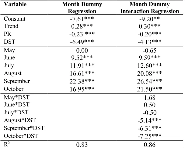
Table 2 shows the results of two DD regression models of household electricity

consumption. Both models are based on equation (4), they include a time trend, and dummies to

control for month effects. In the first model, we assume that the effect of DST on electricity

consumption is the same for all DST months. In the second model, we include interactions

between the month dummies and DST. Therefore, we can test whether DST has different effects

on different months.

Table 2. Domestic Electricity Consumption Results (pooled regression)

Variable Month Dummy Regression

Month Dummy Interaction Regression

Constant -7.61*** -9.20**

Trend 0.28*** 0.30***

PR -0.23 *** -0.20***

DST -6.49*** -4.13***

May 0.00 -0.65

June 9.52*** 9.59***

July 11.91*** 12.60***

August 16.61*** 20.08***

September 22.38*** 26.54***

October 16.95*** 21.50***

May*DST (dummy)

1.68

June*DST 0.50

July*DST -0.50

August*DST -5.14***

September*DST -6.31***

October*DST -7.25***

R2 _{0.83 0.86}

*,** and *** indicate that the coefficient associated with the DLS dummy variable is significant at 10% , 5% and 1%, respectively.

All the coefficients in the regressions have the expected signs. First, the trend coefficient

is positive. This means that DST consumption of electricity is growing faster than non-DST

consumption. As mentioned before, this is probably explained by warmer summers; as well as an

increase in the availability and use of air conditioning (AC) with time. Second, the price

coefficient is negative. That is, an increase in the price difference between treatment and control

months, reduces the difference in consumption of electricity. However, the effect of this variable

is small; suggesting that household demand for electricity is relatively price inelastic. Third, the

10

important to highlight that DST has a smaller effect on consumption during the first four months

of the period (that is, April, May, June, and July) in comparison with the last three months

(August, September, and October).

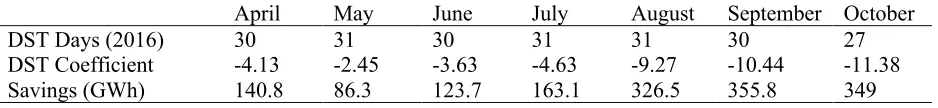
We can use the model to calculate electricity savings due to DST. Note that is the

effect of DST on electricity consumption. However, the DST coefficient that we estimate in the

regressions is . Given that (that is, average daily consumption in non-DST months)

was about 113.6 GWh during year 2016, the effect of DST in a given month is .

Finally, we should multiply the corresponding figure by the number of DST days in the month to

estimate monthly savings.

Table 3. Estimated DST electricity savings in year 2016

April May June July August September October DST Days (2016) 30 31 30 31 31 30 27 DST Coefficient -4.13 -2.45 -3.63 -4.63 -9.27 -10.44 -11.38 Savings (GWh) 140.8 86.3 123.7 163.1 326.5 355.8 349

Table 3 shows estimated electricity savings for each month in year 2016. The DST

coefficients that we use come from the pooled regression with interaction terms. Therefore, DST

coefficients vary with the month. Electricity savings due to DST in the whole period are 1,545.1

GWh. Given that total electricity consumption in the country was about 260 thousand GWh in

year 2016, DST savings in residential electricity consumption represent almost 0.6% of total

electricity consumption in Mexico.

We use the same procedure to estimate electricity savings due to DST both in the middle

of the 90s (when DST was introduced in Mexico) and about ten years later. These estimates can

be compared to previous estimates obtained by Ramos et al. (1998) and Maqueda and Rebolledo

(2008), respectively. Average daily consumption by households was about 68.9 GWh in the

1996. Therefore, yearly savings generated by DST were about 937.1 GWh. This number was

approximately 0.7% of total electricity consumption in the country at that time. Note that it is

almost twice the savings we calculated with a simple DD comparison in the previous section.

Moreover, this number is in line with the estimates obtained by Ramos et al. (1998). Similarly,

considering that daily household consumption was about 93.4 GWh in 2008, we can estimate

g

o

Q c 100

g

= Qo

136 . 1 ´ =c

11

that savings generated by DST were around 1,270 GWh at that time. This figure is about 14%

larger than the 1,115 GWh savings estimated by Maqueda and Rebolledo (2008).

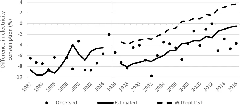
Fig. 2A. Effect of DST on electricity consumption: April vs. Non-DST months

Figure 2A illustrates the effect of DST in a particular month. The dispersed square-dots

in this figure are observed differences in daily consumption between April and the average of

non-DST months at different points in time. Daily electricity consumption in this month is

usually smaller than the average of non-DST months. Nevertheless, it is clear that this difference

is becoming smaller over time. That is, this difference has a positive trend. The thin vertical line

indicates the moment in which DST started in Mexico. The increasing solid line is the difference

in electricity consumption (between April and non-DST months) predicted by the model. The

dotted line is what the model predicts without DST. Although DST reduces consumption in

April, this effect is relatively small.

Although we are using essentially a DD approach, it is worth mentioning that Figure 2A

resembles the ones that are typically obtained with regression discontinuity (RD) analysis. As

explained by Thistlewaite and Campbell (1960), who used RD originally to measure the effects

of an award on student attitudes toward intellectualism, the treatment must cause a jump in the

regression line plots at the cutting point. In Thistlewaite and Campbell (1960), the cutting point

is the arbitrary minimum test score required to obtained the award. In this case, the cutting point

is the year in which the Mexican government decided to start implementing DST in the country.

-10 -8 -6 -4 -2 0 2 4

1982 1984 1986 1988 1990 1992 1994 1996 1998 2000 2002 2004 2006 2008 2010 2012 2014 2016

Di

ff

e

re

n

ce

i

n

e

le

ct

ri

ci

ty

consum

pt

ion

(%

)

12

It is worth mentioning that regression discontinuity analysis is used by Toro, Tigre and Sampaio

(2015) to evaluate the effects of DST on myocardial infarction.

Fig. 2B. Effect of DST on electricity consumption for different DST months vs. Non-DST months

The effect of DST on electricity consumption varies throughout the months in which the

program is in effect. Figure 2B shows the effect of DST from May to October. It is worth making

a couple of comments about these graphs. First, daily electricity consumption during most DST

months has been larger than consumption during non-DST months both before and after DST

started. Second, there is a positive trend in the difference between consumption in each DST

month and average consumption in non-DST months. That is, electricity consumption in DST

months has been growing faster than consumption in non-DST months. Finally, the effects of

DST seem to be substantially larger in the last three months of DST (that is, August, September,

and October) in comparison with the first three months (that is, May, June, and July).

-12 -7 -2 3 8

1982 1986 1990 1994 1998 2002 2006 2010 2014

Di ff e re n ce (% ) May -4 1 6 11 16

1982 1986 1990 1994 1998 2002 2006 2010 2014

June -2 3 8 13 18

1982 1986 1990 1994 1998 2002 2006 2010 2014

July 0 5 10 15 20 25

1982 1986 1990 1994 1998 2002 2006 2010 2014

Di ff e re n ce ( % ) August 4 14 24 34

1982 1986 1990 1994 1998 2002 2006 2010 2014

September Observed Estimated Without DST -2 3 8 13 18 23 28

1982 1986 1990 1994 1998 2002 2006 2010 2014

13 5. Robustness checks

In this section, we present the results of four robustness checks. First, we include

dummies to control for the four large economic crises that took place in Mexico during the

period under study. Second, we introduce placebo beginnings of DST. That is, we arbitrarily

move the beginning of DST to the middle of the periods before and after it was actually

implemented. Third, we run separate regressions for DST months, using the average of the

non-DST months as the control group. Fourth, we run again separate regressions for non-DST months,

using now electricity consumption in a single non-DST month as a control instead of an average

of all non-DST months.

5.1. Controlling for large economic crises

In principle, the method that we use to estimate the effects of DST on residential

electricity consumption should be immune to economic cycles. We are using an average of

electricity consumption during non-DST months as controls. It is unlikely that only DST months

or non-DST months, in a given year, are affected by an economic expansion or a recession.

Moreover, transitory changes in income should have small effects on consumption.

Nevertheless, it is worth checking whether large economic crises –like the ones that occurred in

Mexico during the period of study– affect the main results of the paper.

The four large economic crises that we are considering in this exercise took place in

1983, 1986, 1995, and 2009, respectively. The Mexican GDP fell at least 3% in each of these

years. We are particularly concerned by the large economic crisis that occurred just one year

before the implementation of DST (that is, the crisis of 1995). The GDP fell more than 6% in

that year. Therefore, it is reasonable to believe that DST may be capturing, at least partially, the

effect of this event.

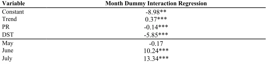
Table 4. Domestic Electricity Consumption Results (pooled regression with recession dummies)

Variable Month Dummy Interaction Regression

Constant -8.98**

Trend 0.37***

PR -0.14***

DST -5.85***

May -0.17

June 10.24***

14

August 20.78***

September 27.18***

October 21.88***

May*DST (dummy)

2.14

June*DST 0.78

July*DST -0.38

August*DST -4.97***

September*DST -6.05***

October*DST -7.19***

1983 -1.09

1986 0.18

1995 -7.56***

2009 3.77***

R2 _0.88

*,** and *** indicate that the coefficient associated with the DLS dummy variable is significant at 10% , 5% and 1%, respectively.

Table 4 shows the results of a pooled regression that includes dummies for the years in

which Mexico suffered large economic crisis. Only the crises of 1995 and 2009 have a

significant effect on the difference in electricity consumption between DST months and

non-DST months. However, they have opposite signs. More importantly, including these controls

does not change qualitatively the main results of the paper. We estimate that DST savings with

these controls are 1,908.7 GWh. This represents 0.73% of total electricity consumption in the

country.

5.2. Placebo effects

Another way to check that our results are robust is to run pooled regressions with placebo

beginnings of DST. With this idea in mind, we create dummies as if DST started in 1989 and

2006, respectively. It is important to say that 1989 is in the middle of the period 1982-1996 and

2006 in the middle of the period 1996-2016. We run two regression using these dummies,

respectively, instead of the dummy for 1996, when DST was actually introduced in Mexico.

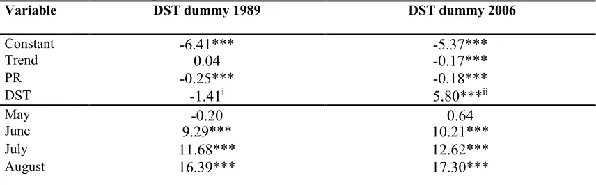
Table 5. Placebo Test Regressions

Variable DST dummy 1989 DST dummy 2006

Constant -6.41*** -5.37***

Trend 0.04 -0.17***

PR -0.25*** -0.18***

DST -1.41i 5.80***ii

May -0.20 0.64

June 9.29*** 10.21***

July 11.68*** 12.62***

15

September 22.17*** 23-06***

October 16-83*** 17.30***

R2 _{0.80 0.83}

*,** and *** indicate that the coefficient associated with the DLS dummy variable is significant at 10% , 5% and 1%, respectively. i DST is zero from years 1982 to 1988 and one afterwards. ii DST is zero from years 1996 to 2005 and one afterwards.

Table 5 shows the results of placebo tests. As expected, the coefficient of the fictitious

DST beginning in 1989 –that is, before the actual beginning of DST– is negative but not

statistically significant. In contrast, the coefficient of the fictitious DST beginning in 2006 –that

is, after the actual beginning of DST– is positive and statistically significant. However, it is

important to note the small negative trend in this regression. This suggests that the fictitious DST

is taking the effect of fast growing electricity consumption in DST months (compared to

non-DST months) that we observe in the data. Finally, we should mention that none of the placebo

DST tests produce electricity savings as the actual DST test.

5.3. Separate regressions for DST months

We can also check the robustness of our results by running separate regressions for each

DST month instead of a pooled regression. The advantage of separate regressions is that each

model may adjust better to the data of the corresponding month. However, the big disadvantage

of separating DST months is that we run regressions with small number of observations.

Therefore, it is harder to find significant effects.

Table 5 shows the results of the separate regressions of household electricity

consumption for the different DST months. Most of the coefficients have the expected signs.

However, some of them are no longer significant. In particular, note that DST has no effect on

consumption during the first two months of DST (that is, April and May). This is not surprising

given that we have a small number of observations; and we know from previous regressions that

DST has a small effect at the beginning of the period.

Table 5. Domestic electricity consumption regressions results for DST months

Variable April May June July August September October

Constant -8.40*** -9.04*** 0.61 2.05 8.32*** 16.59*** 12.99*** PR 0.06 -0.04 -0.07 -0.23* -0.48*** -0.32* -0.20 TREND 0.24*** 0.39*** 0.49*** 0.44*** 0.14 0.19 0.18 DST -1.55 -2.06 -5.75** -7.45** -8.99*** -9.84*** -9.45*** R2 0.40 0.6 0.52 0.46 0.51 0.38 0.40

16

We can use the estimates obtained in this model to calculate again domestic electricity

savings due to DST in year 2016. According to these results, yearly savings generated by DST

are about 1,525.5 GWh. These savings are slightly lower than our initial estimate. However, they

still represent about 0.6% of total electricity consumption in the country.

5.4. Single months as controls

We run again separate regressions for DST months. However, we now use electricity

consumption in a single non-DST month as a control instead of an average of all non-DST

months. The most natural controls for this robustness check are months adjacent to the treatment

months (that is, March and November). In particular, we believe that March is a better control

than November. In several ways, March is closer to summer months than November. Karasu

(2010) points out that the change in the average temperature in Turkey from March (without

DST) to April (with DST) is marginal (it increases 2.2 degrees C), while the change in

temperature from October (with DST) to November (without DST) is large (it decreases 7.6

degrees C). Something similar occurs in Mexico. For instance, there are about 11:45 hours of

sunlight in Mexico at the beginning of March. In contrast, there are only about 11:00 hours of

sunlight at the end of November. Nevertheless, we will use each of the non-DST months as

control and show all the results.

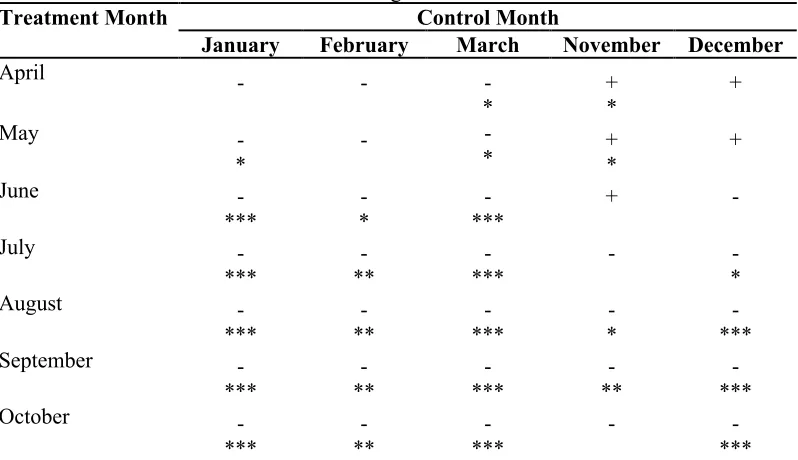
Table 6. DST effect on treatment months using different months as controls

Treatment Month Control Month

January February March November December

April _{- - -}

* + * + May _- * - - * - + * +

June _- *** - * - *** + -

July _- *** - ** - *** - - * August _-

*** - ** - *** - * - *** September _-

*** - ** - *** - ** - *** October _-

*** - ** - *** - - ***

17

We summarize the main results of this last robustness check in Table 6. Basically, we

specify the sign of the DST coefficient (whether it resulted positive or negative) for each

combination of months; and its level of significance. Regardless of the month that we use as

control, we cannot reject –with a 5% level of significance– the null hypothesis that DST has no

effect on electricity consumption in April and May. Moreover, only if we consider March as the

control month, we find that DST reduces consumption in these two months at a 10% level of

significance. However, we obtain the exact opposite result (that is, that DST increases electricity

consumption) if we use November as the control month. Therefore, these results suggest that

DST generates small savings –if any– in electricity consumption during the beginning of DST.

On the other hand, we reject the null hypothesis that DST has no effect on consumption –with a

1% level of significance– for each month from June to October if we use the months of January

and March as controls. Similarly, we reject the null hypothesis that DST has no effect on

consumption –with a 5% level of significance– from July to October if we use February as

control; or with a 1% level of significance from August to October if we use December as

control. Hence, there is sufficient evidence to say that that DST reduces consumption of

electricity towards the end of the DST period.

6. Conclusion

In this paper, we evaluate econometrically whether DST reduces or not household

electricity consumption in Mexico. We use time series data and a DD approach in order to

estimate savings generated by DST at different points in time. According to our estimates, DST

has been reducing domestic electricity consumption in Mexico since the program started in 1996.

Moreover, we find that DST reduces electricity consumption nowadays by 1,545.1 GWh on a

yearly basis. These savings account for 0.6% of total electricity consumption in the country. It is

important to mention that this figure is in line with previous estimates in Mexico; and large in

comparison to the 0.34% mean of the literature reported in the meta-analysis elaborated by

Havranek, Herman and Irsova (2018).

We also find that DST does not reduce consumption homogeneously during the whole

18

DST generates larger savings towards the last months (August, September, and October) of the

period. This result contrasts with the previous findings of Momani, Yatim and Ali (2009) for

Jordan. They recommend not implementing the DST in September (that is, towards the end of

the DST period in Jordan).

The fact that we find some evidence that DST has relatively smaller effect on household

electricity consumption during the first months of the period, is not sufficient to conclude that the

authority should shorten the duration of DST in Mexico. There are several reasons not to do it.

First, there is no strong evidence to say that DST increases electricity consumption in any

particular month. Second, even if DST does not reduce residential electricity consumption in a

given month, it may still smooth consumption during the day generating savings in the

production of electricity. Third, given the commercial links between Mexico and the US, it

benefits to coordinate on the DST as much as possible.

Acknowledgment

The authors declare that they have no conflict of interest and that no particular funding was

received in order to write this manuscript.

References

Ahuja, D.R., Sengupta, D.P., 2012. Year-round daylight saving time will save more energy in

India than corresponding DST or time zones. Energy Policy 42, 657-669.

Angrist, J.D., Pischke, J.S., 2009. Mostly harmless econometrics: An empiricist’s companion.

Princeton University Press: Princeton.

Aries, M., Newsham, G.R., 2008. Effect of daylight saving time on light energy use: a literature

review. Energy Policy36, 1858-1866.

Choi, S., Pellen, A., Masson, V., 2017. How does daylight saving time affect electricity demand?

An answer using aggregate data from a natural experiment in Western Australia. Energy

Economics 66, 247-260.

Ebersole, N., Rubin, D., Hannan, W., Darling, E., Frenkel, L., Prerau, D., Schaeffer, K., 1974.

The year-round daylight saving time study. Interim Report on the Operation and Effects

19

Havranek, T., Herman, D., Irsova, Z., 2018. Does daylight saving save electricity? A

meta-analysis. Energy Journal 39, 35-61.

Her Majesty’s Stationary Office, 1970. Review of British Standard Time. Number 4512. British

Government.

Hill, S.I., Desobry, F., Garnsey, E.W., Chong, Y.-F., 2010. The impact on energy consumption

of daylight saving clock changes. Energy Policy 38, 4955-4965.

Kandel, A., Sheridan, M., 2007. The effect of early daylight saving time on California electricity

consumption: a statistical analysis. California Energy Commission Staff Report

CEC-200-2007-004.

Karasu, S., 2010. The effect of daylight saving time options on electricity consumption of

Turkey. Energy 35, 3773–3782.

Kellogg, R., Wolff, H., 2008. Daylight time and energy: Evidence from an Australian

experiment. Journal of Environmental Economics and Management56, 207-220.

Kotchen, M.J., Grant, L.E., 2011. Does daylight saving time saves energy? Evidence from a

natural experiment in Indiana. Review of Economics and Statistics93, 1172-1185.

Marshall, D., 2010. El consumo eléctrico residencial en Chile en 2008. Cuadernos de Economía

47, 57-89.

Maqueda, M.R., Rebolledo, H.P., 2008. Metodología de evaluación del Cambio de Horario de

Verano (CHV) en México: 10 años de aplicación. Boletín IIE 32(1): 9-18.

Mirza, F.M., Bergland, O., 2011. The impact of daylight saving time on electricity consumption:

Evidence from southern Norway and Sweeden. Energy Policy39, 3558-3571.

Momani, M.A.,Yatim, B., Ali, M.A., 2009. The impact of daylight saving time on electricity

consumption-A case study from Jordan. Energy Policy37, 2042-2051.

Ramos, G.N., Covarrubias, R.R., Sada, J.G., Buitron, H.S., Vargas, E.N., Rodriguez, R.C., 1998.

Energy saving due to the implementation of the daylight saving time in Mexico in 1996.

In: Proceedings of the International Conference on Large High Voltage Electric Systems,

vol. 13.

Shimoda, Y., Asahi, T., Taniguchi, A., Mizuno, M., 2007. Evaluation of city-scale impact of

residential energy conservation measures using the detailed end-use simulation model.

20

Toro, W., R. Tigre, Sampaio, B.,2015. Daylight Saving Time and incidence of myocardial

infarction: Evidence from a regression discontinuity design. Economics Letters136:

1361-1364.

Thistlewaite, D.L., Campbell, D.T. 1960. Regression-Discontinuity analysis: An alternative to

the ex-post facto experiment. Journal of Educational Psychology 51, 309-317.

Verdejo, H., C. Becker, D. Echiburu, W. Escudero, Fucks, E., 2016. Impact of daylight saving