Munich Personal RePEc Archive
Comparing votes and seats with cosine,
sine and sign, with attention for the
slope and enhanced sensitivity to
inequality / disproportionality
Colignatus, Thomas
Thomas Cool Consultancy Econometrics
9 February 2018
Comparing votes and seats with cosine, sine and sign, with
attention for the slope and enhanced sensitivity to inequality /
disproportionality
Thomas Colignatus
September 16 2017 & February 9 2018
JEL
A100 General Economics: General
D710 Social Choice; Clubs; Committees; Associations,
D720 Political Processes: Rent-seeking, Lobbying, Elections, Legislatures, and Voting Behavior
D630 Equity, Justice, Inequality, and Other Normative Criteria and Measurement
MSC2010
00A69 General applied mathematics
28A75 Measure and integration. Length, area, volume, other geometric measure theory 62J20 Statistics. Diagnotics
97M70 Mathematics education. Behavioral and social sciences
Abstract
Let v be a vector of votes for parties and s a vector of their seats gained in the House of Commons or the House of Representatives. We use a single zero for the lumped category of "Other", of the wasted vote, for parties that got votes but no seats. Let V = 1'v be total turnout and S = 1's the total number of seats, and w = v / V and z = s / S the perunages (often
percentages). There are slopes b and p from the regressions through the origin (RTO) z = b w
+ e and w = p z + ε. Then k =Cos[v, s] = Cos[w, z] = Sqrt[b p]. The geometric mean slope is a symmetric measure of similarity of the two vectors. θ = ArcCos[k] is the angle between the vectors. Thus Sin[v, s] = Sin[w, z] = Sin[θ] = Sqrt[1 – b p] is metric and a measure of disproportionality in general. Geometry appears to be less sensitive to disproportionalities than voters, representatives and researchers tend to be. This likely relates to the Weber-Fechner law. Covariance gives a sign for majority switches. A disproportionality measure with enhanced sensitivity for human judgement is the sine diagonal inequality/disproportionality
SDID = sign 10 √Sin[v, s]. This puts an emphasis on the first digits of a scale of 10, which can be seen as an inverse (Bart Simpson) report card. What does disproportionality measure ? The unit of account can be either the party or the individual representative. This distinguishes between the party average and the party marginal candidate. The difference z – w is often treated as a level, and Webster / Sainte-Laguë (WSL) uses the relative expression z / w – 1. For the party marginal candidate z – w already is relative, with the unit of account of the individual representative in the denominator. The Hamilton Largest Remainder (HLR) apportionment has the representative as the unit of account. The "Representative Largest Remainder" (RLR) uses a 0.5 natural quota. The paper provides (i) theoretical foundations, (ii) evaluation of the relevant literature in voting theory and statistics, (iii) example outcomes of both theoretical cases and the 2017 elections in Holland, France and the UK, and (iv)
comparison to other disproportionality measures and scores on criteria. Using criteria that are accepted in the voting literature, SDID appears to be better than currently available
measures. .
Keywords
General Economics, Social Choice, Social Welfare, Election, Majority Rule, Parliament, Party System, Representation, Sine Diagonal Inequality / Disproportionality, SDID, Proportion, District, Voting, Seat, Euclid, Distance, Cosine, Sine, Gallagher, Loosemore-Hanby, Sainte-Laguë, Webster, Gini coefficient, Lorenz, Jefferson, Hamilton, Largest Remainder,
1. Introduction ...4
1.1. Overlapping chapters in Social Choice and Public Choice ...4
1.2. The literature and what we will do ...8
1.3. Much Ado About Nothing...9
1.4. Statistics and heuristics on the slope ...11
1.5. Electoral justice and inequality ...11
2. Graphs of (half) election results in 2017 in Holland, France and UK ...12
3. Different purposes in voting literature and statistics in general ...14
3.1. Descriptive statistics and decisive apportionment...14
3.2. Different models and errors ...15
3.3. A role for cosine and sine ...16
3.4. Disproportionality, dispersion and education...17
3.5. A bit more formal ...18
4. Definition of SDID and graphical comparison with ALHID, EGID, WSL...19
4.1. Definition of the SDID measure...19
4.2. Weber-Fechner consideration ...20
4.3. The properties for a metric are satisfied...21
4.4. Example of failure rate decomposition ...21
4.5. Graphical comparison of SDID, ALHID, EGID and WSL ...22
4.6. Scores for Holland, France and UK in 2017...25
5. Spaces: vector and 2D scatter, and unit simplex and its 2D scatter ...27
5.1. Notation ...27
5.2. The unit simplex ...28
5.3. Angles, Cos, Sin and Tan...28
5.4. Angular distance measure θ...29
5.5. Example of the Ternary Plot ...30
5.6. Weber-Fechner for angles...31
5.7. The choice on angle and slope measures...32
6. Principles: What are we measuring ? ...32
6.1. The Status Quo and the meaning of the majority rule...32
6.2. Unit proportionality as a power preserving rule ...33
6.3. The unit of account: voter, representative, party, state ...33
6.4. A method of measuring ...34
6.5. Reasons for measuring ...35
6.6. Specific and nonspecific factors, inside or on top ...35
7. Decomposition of "sine diagonal inequality / disproportionality" (SDID) ...36
7.1. Regression through the origin with variables on the unit simplex ...36
7.2. True variables v* and s* and particular observations v and s ...36
7.3. Cos, slope and concentrated numbers of parties...36
7.4. Analyses of squares for the direct error ...38
7.5. Specific and nonspecific disproportionality...39
7.6. Decomposing the SDID measure...39
8. Investigating a potential bias of SDID for HLR, relation of errors to remainders...40
8.1. Comparing on Balinksi & Young 1975 cases ...40
8.2. Fundamental property: remainder → error → Euclidean distance → Sine...41
8.3. An aspect of symmetry...42
8.4. Tie-breaking...43
8.5. Seat transfer when votes are given...43
8.6. Vote transfer when seats are given: decomposition on w and r...44
8.7. Within the locus of apportionment ...48
8.8. General error ...50
8.9. Behaviour of numerator and denominator of Cos ...50
9. Definition of the "sine – target-slope deviation" (STSD) measure (on top of sine)...52
9.1. When the sine is insufficiently sensitive to a target slope ...52
9.2. Test application of STSD for Holland 2017 ...53
10. Heuristic of the measure: error around the slope of 1...54
10.1. Symmetry and normalisation of the input: key step in the definition...54
10.2. Variance ratio and the F-test...55
10.3. (Dis-) Advantages of Pearson correlation...56
10.4. Regression through the origin: key step in the definition...57
10.5. Normalisation of the output: key step in the definition ...58
10.6. Restatement of diagonal regression, major axis, geometric mean functional relationship, or neutral regression...58
10.7. Relation to the cosine: key step in the definition...59
10.8. Relation to Hirschman-Herfindahl or Taagepera-Shugart ENP / CNP ...60
10.9. Weighed regression ...60
10.10. Thus the sine diagonal inequality / disproportionality (SDID) measure...61
11. Apportionment, measuring, wasted vote...61
11.1. Definition of "wasted vote" ...61
11.2. Apportionment (Jefferson, Webster, Hamilton)...62
11.3. Inequality / disproportionality measures based upon apportionment ...65
11.4. Statistical measures: Kullback-Leibler (KL) and Chi square...65
11.5. Correlation and cosine ...66
11.6. Euclid / Gallagher distance (EGID) and cosine ...68
11.7. A measure that uses the determinant...69
11.8. Can a uniform best measure be based upon tradition ?...69
12. Comparison of scores on theoretical cases ...69
12.1. Comparison of bipartite cases around 50%...70
12.2. Comparison of bipartite cases with a small party ...71
12.3. Comparison of bipartite cases with a tiny party ...71
12.4. Comparison of tripartite cases ...72
12.5. Comparison of quadripartite cases ...74
12.6. Comparison on the Dalton transfer...75
13. Scoring on the Taagepera – Grofman criteria...77
14. Conclusion...79
15. Appendix A. Abstract of Colignatus (2017b) ...82
16. Appendix B. Some comments on the unit simplex...82
16.1. EGID and Origin Concordance (OC) ...82
16.2. Aitchison geometry ...83
17. Appendix C. Using Abs[k – 1 / k] and another transform...83
18. Appendix D. Xur & Yur ...84
19. Appendix E. The average...85
20. Appendix F. Potential use for apportionment, Holland 2017 ...86
21. Appendix G. Normalisation of T, b and p on unit circle...87
22. Appendix H. Cos[z / w, 1] allows undesirable compensation ...88
23. Appendix I. Major revision...90
24. Appendix J. Target base parameters and STSD ...90
24.1. A misleading heuristical idea ...91
24.2. Model with a general target T*...91
24.3. Relevance for votes and seats: the example of turnout ...92
24.4. Is the error on the target additional or already included ? ...92
25. Appendix K. Failures on failure rate decomposition...94
25.1. SST = SSX + SSE ...94
25.2. The Hirschman-Herfindahl concentration index...95
25.3. Cos = √(b p) = b √(w'w / z'z) ...95
25.4. On overall strategy for looking into this...95
26. Appendix L. Representative Largest Remainder (RLR), Holland 2017 ...96
27. Appendix M. The effect of the number of seats on HRL and RLR...98
28. Appendix N. Relation of HLR, RLR and ALHID, "New State Paradox" ...100
29. Appendix O. Update February 6 2018 ...101
1. Introduction
1.1. Overlapping chapters in Social Choice and Public Choice
This paper falls in the category of Public Choice, as defined by Gordon Tullock (2008) as "the use of economic tools to deal with traditional problems of political science" (JEL D710 and D720). We will also present a new disproportionality index based upon cosine and sine, which falls in a different category (JEL D630). Overall the general content is large (JEL A100).
Economics has a main stream that adopts "methodological individualism". This assumes that explanations are sought in the behaviour of individuals, as opposed to assuming units like
The Family or The State. In Idealism, for example, one might imagine that The State is "an entity" with a life of itself. This would be Idealism and not economics. Similarly for the question whether The Party can be a unit of account in votes and seats. In the USA there is
apportionment of seats in the House of Representatives for the States of the Union, with the current method of Huntington – Hill. 1 Populations link up with States and it makes sense to
use these as units of account. 2 For parties it is different. These are voluntary coalitions of voters and their representatives. Methodology requires that we look at the individual unit of account rather than The Party. In this case, the unit thus is the party marginal candidate. For economists, the notion of marginal analysis may have an additional appeal.
Politicians, their bureaucracies and the scientists and mathematicians hired for such purposes, have been adopting particular conceptions or psychological frames, which in science might be called a paradigm. In this case, it is the adoption of The Party as the unit of account. This causes such collusion and confusion, that perhaps even scientists no longer are fully aware of what is happening. Thus we need to construct both (i) what really is at stake and (ii) what that paradigm is, that causes such confusion about what really is at stake.
There is the distinction between Equal or Proportional Representation (EPR) and District Representation (DR). Carey & Hix (2009) (2011) discuss the optimal district magnitude, i.e.
the number of seats per district. They perceive a trade-off or balance of accountability and representation, and rely on the Euclid / Gallagher Inequality / Disproportionality (EGID) measure for their regressions. There are various issues with their analysis that receive attention in Colignatus (2017d). For this present paper, it suffices to say that C&H overlook that DR appears to be fraught with error and mishap, and that EGID is somewhat dubious. Because of the mishap of DR, Holland in 1917 switched to EPR. Somehow, the UK, USA and much of the English Speaking World (like India) missed the boat. This has been causing a lot of trouble to the world. What causes it, that scientists do not clearly explain to politicians and the public that DR is disastrous, and that EPR is the approach that is required by both intellectual integrity and social harmony ? Apparently Carey & Hix (2011) point to
accountability, but as said, this is discussed by Colignatus (2017d). The present focus is on inequality / disproportionality measures, that form part of this paradigm of confusion.
Indeed, in the UK there is the Electoral Reform Society (ERS), that advocates a system called "Single Transferable Vote" (STV), that they call EPR but that is not EPR because it still links up to the UK tradition of DR. Such notions at ERS were historically caused by the same concerns that caused Holland in 1917 to switch to EPR. Thus there is scope for progress. It is tragic that this scope gets bogged down in other swamps, in this case at ERS in the confusion about STV. (A confusion is too that voters should use such more complicated methods. Instead, voters best vote for an EPR party list system, while the professionals in parliament might use more complex systems.)
We now look at a part in the literature about measures of inequality / disproportionality. It appears that reseachers have built a cathedral of misconceptions here as well. We need to deconstruct this cathedral and show what really is at stake.
1 Young (2004) in a symposium at the US Census Bureau argues rather convincingly that
advanced insight shows that Webster would be better. See also Balinski & Young (1980).
2 Alexander Bogomolny has online routines:
In the USA, interest for disproportionality only concerned the allocation of seats to States, as said, which resulted into the Huntington – Hill method (see footnote 1). The USA has no interest in EPR itself since they have a system with DR. When Arend Lijphart moved from Holland to the USA, he took along a support for the notion of EPR, which he even called
electoral justice. However, he may also have been sensitive to his new environment of DR, for apparently Lijphart also started to embrace The Party, and thus may have overlooked a key aspect of EPR that we now will highlight, namely equal representative democracy.
Obviously, when we would inform the decision makers and public in the USA, UK or France about the advantages of EPR, then the system should be a proper improvement over their current systems. Even Holland is not as EPR as can be.
We consider a vector v of votes, with a total number of votes V = 1'v (turnout). The length of the vector is the number of parties n. The vector s of the seats has a total number of seats S
= 1's. There are shares or proportions w = v / V and z = s / S, unitised to 1 onto the unit simplex so that 1'w = 1'z = 1. A common use is 100 percent, but this may suggest overly precision, and 10 suffices to get rid of the leading zeros.
Table 1 contains an example. It shows how V = 325 voters elect S = 10 seats. The electoral quota is Q = V / S. Dividing the votes by the quota gives a as the average number of seats that a candidate can claim, a = v / Q = S v / V = S w. The locus of apportionment of seats s is Floor[a] ≤ s ≤ Ceiling[a], or the averages rounded down or up to the nearest integer. The first batch of seats that can be allocated is Floor[a]. This generates 9 seats that can be assigned directly. There is 1 remainder, and at issue is what principle shall be used to assign this. At issue is not the particular method, but the principle. What defines equal (proportional) representative democracy ? The question is whether the unit of account is the party or the
individual representative, here the party marginal candidate. The method of highest averages
would better be called the method of highest artificial ratios, since Methodological
Individualism requires attention for the individual level and not the assumption of The Party.
Table 1. Unit of account: Voter and (representative versus party)
Methodological Individualism versus
Party as a unit of account (marginal candidate)Largest remainder "Highest average"(party as unit)
Party Votes v v / Q Floor[v/Q] Remainder Seats s v / (Floor+1) Seats s
John 25 0.77 0 0.77 1 25.00 0
Blue 100 3.08 3 0.08 3 25.00 3
Green 200 6.15 6 0.15 6 28.57 7
Total (V, S) 325 10 9 10 10
Q = V / S 32.5 (Electoral quota)
Let there be K candidates with vKvotes for the candidates. Elected are sK. There are n
parties. Then G is a {n, K} aggregation matrix with 0 and 1, so that v = G vKand s = G sK are
the aggregate outcomes for parties, in which an independent individual can be called a party by himself or herself. This administration should not cause us to use The Party as the unit of account. For we should rather look at the party marginal candidate.
Comments w.r.t. Table 1 are:
(1) In Methodological Individualism, individual candidate John is not opposed to the other parties, but to the candidates in those parties. The remainder seat does not concern the parties but their marginal candidates. The party list determines which particular candidate.
(a) The relevant principle is "votes per candidate" or the Remainder Divided By 1 Candidate. In voting research this is often seen as a level difference, but it is a ratio, with the marginal candidate in the denominator.
(c) There are K candidates and V / K votes per candidate on average. The parties manage to collaborate, and collect their remainders, so that more of them can be elected. Their benefit should not be an argument to cause a loss to others. (d) It is a difficult issue how to handle inequal votes within a party, but it is accepted
practice, and indeed not unreasonable for the formation of coalition governments, that parties can combine their votes into the Floor value. The Floor apportionment fully satisfies the quota and thus can drop from inequality / disproportionality measures, so that these measures can concentrate only on the remainder seats. (e) It would be another step to accept that parties can also claim more than this. As
said, their advantage should not be construed to cause a loss to others.
(f) What about "extreme situations" ? If John got only 2 votes and the other parties had only marginal votes 1 each, then HLR would cause him to be elected (if the electoral quota allowed such small margins, while taking into account that the fractions must add up to the remainder seats). The votes for the larger parties indicate that their remainders are somewhat part of chance processes, while John faces the existential question. To deal with this kind of issue, it is not unreasonable to set a threshold of say 50% of the electoral quota, applicable only to the
allocation of the remainder seats. The number is arbitrary, except for the
expectation that fractional remainders might tend to average around 50% of a seat. The norm that the fraction ≥ 0.5 fits the convention to round up (compared to the strictness of > 0.5).
(g) This situation also clarifies the rise of parties. Perhaps a short example helps. If such a threshold would be 0.5 Q and there would be 21 candidates who all got a 10 / 21 share of the vote, then none would pass (325 / 21 / Q). There is an obvious advantage that there are parties who collect the remainders. But an advantage for parties should not necessarily work against those not in a party system, who do not need to collaborate and still get at least 0.5 Q. Said in another way: with such 10 / 21 outcome, there would arise bargaining amongst the candidates, who would be elected, and this explains the rise of parties. Yet this should not merit the adoption of The Party as the unit of account.
(2) When parties are taken as the unit of account (with similar methods as taking States as the unit of account), then it makes some sense to look at the average votes per seat.
(a) The Floor and the assigned seats already satisfy the electoral quota Q. For each party we can look at what would happen to the ratio of "votes per seat" when that party would get another seat. John has 25 votes and thus a ratio of 25. The Green party has a small remainder of 5 votes, with 5 / 32.5 ≈ 0.15, but the party is so large that the addition of 1 seat still generates a high average of "votes per seat" for that particular party. In this case Green generates the highest average. This philosophy assigns the remainder to them.
(b) Sometimes the party system is enhanced by requiring a higher threshold. If the number of seats is large then there is much to be said for the natural threshold of the electoral quota. Yet case (1) above shows that candidates below the natural quota can do better than the marginal candidates in parties. One should have a very good reason to exclude the small independent voice.
(c) The argument in favour of parties is that they represent an ideology, and that voting rather concerns party programs than individual representatives. Perhaps. It is not clear though that this is a good reason to exlude the small independent voice that has a higher vote than the party marginal candidate.
For example, Balinski & Young (1976:17-18) present above party-quota rule. What they effectively do is to replace Hamilton's "votes per seat" into "votes per party seats". They argue correctly that a choice on electoral systems should be based upon criteria, but they present criteria based upon parties and not upon individual representatives. They state:
representation systems in that it inferentially asks for a "large" vote before according any representation at all."
They think in terms of The Party and overlook Methodological Individualism. Their background is in mathematics and not in economic theory.
Appendix L shows that the issue is relevant for Holland 2017. The Dutch system is perhaps the most proportional in the world but can still be improved. Appendix M shows the difference between HLR (without threshold) and RLR (with at least 0.5 Q for remainder seats).
The latter appendix also shows the effect of the number of seats S. The literature on inequality / disproportionality measures tends to compare relative allocations of votes and seats, i.e. w and z, but the number of seats S likely affects our interpretation of the behaviour of the measures. Given that HLR / RLR rather define equal (proportional) representative democracy, for national parliaments of adequate size, we should not be distracted by supposed paradoxes highlighted by examples with low numbers of seats. For countries with DR, this issue on the number of seats is discussed under the label of "district magnitude", while the relevant discussion is actually about replacing DR with EPR.
The focus on properties of different methods of apportionment is also overdone, while the real discussion concerns the shift from DR to EPR. Beumer (2010:57) looks at 16 Dutch elections in th 50-year period of 1956-2006, and finds for the Dutch House of 150 seats:
"Coalitions [ftnt] are always formed with a clear margin over the simple majority of 75 seats. Webster apportionments only shift a small number of seats: on average the difference between a Webster apportionment and a Jefferson apportionment is 3.88 seats on a total of 150. Additionally, the difference is virtually always one seat per party; in the period 1956–2006 there is only one occurrence of a two-seat difference. This means that an average coalition of three parties could typically lose three seats. This is not enough to lose the majority. In particular, Webster with minimum
requirements would have lead to exactly the same coalitions."
Once you discover a statistical regularity, it is in danger of evaporating. It so happens that the new coalition in Holland 2017 has 4 parties with only 1 seat majority. If apportionment were a real conundrum, then one might also assign representatives the weights of the votes that they actually got, above some threshold. There is no urgent need for this, since HLR / RLR work well, and rather define what equal (proportional) representative democracy actually is.
The Political Science literature on apportionment and inequality / disproportionality measures is huge, and they all tend to overlook the above and to adopt the paradigm of The Party. For science it is okay to look at the consequences of a particular hypothesis. However, this literature also comes with the attitude that researchers would be interested in inequality / disproportionality per se. Apparently only within their paradigm of The Party. For authors coming from countries with DR, the issue on such measures may only be a theoretical exercise in mathematics, or an application as in the USA on States. Subsequently, they present a zoo of possible measures. With such confusion, it is relatively easy for decision makers and the public in DR countries to suffer an information overload on EPR, and then remain with DR. If EPR is so difficult to understand, why change ?
Balinski & Young presented an "impossibility theorem" though assumed The Party. Though this only concerns a mathematical result, the effect of choosing such framing is that it creates the suggestion as if a sound system would be impossible, or that it would be impossible to
define what equal (proportional) representative democracy would be. I am reminded of the story of Ignaz Semmelweis (1818-1865). 3 Current Political Scientists with their lack of criticism of DR are similar to doctors who attend to childbirth without washing their hands. Their defence may be that they are no real doctors treating patients but only academic researchers. They still suffer from the paradigm of The Party and thus create all kinds of confusions that prevent the world to adopt EPR like in Holland in 1917. Obviously one would
not indiscriminately copy all that Holland managed to do in 1917, but the present intellectual outrage is the created confusion about the proper formulation of the research issue. It may also be a case of mathematical abstraction running astray, and onlookers not able to perceive what the mathematicians actually are doing but still following their lead.
Our present purpose is to (i) deconstruct the discussion in Political Science about inequality / disproportionality measures, (ii) show what the problem really is (actually already done in the above), (iii) present a clear and simple inequality / disproportionality measure (though with options to make it more complex again). Appendix L contains a representative based
apportionment method, and we continue with the general measurement issue.
1.2. The literature and what we will do
The literature on voting has a rich discussion about potential measures for the inequality / disproportionality of the allocations of s given v. Taagepera & Grofman (2003:673) rightly write about a "zoo of indices proposed and used by various researchers", and they score 19 indices on 12 criteria. 4 Overview discussions are by e.g. Taagepera & Shugart (1989), Gallagher (1991), Taagepera & Grofman (2003), Kestelman (2005), Karpov (2008) and Renwick (2015). Malkevitch (2002) gives a discussion in an AMS feature column. Perhaps for historical reasons this literature has focused on the inequality / disproportionality format, in which 0 indicates equality / proportionality and in which 1 might be full disproportionality - if the measure is normalised on [0, 1]. We also adopt this latter format, though allow for a sign in [-1, 1]. Section 8.1 gives an nicely designed example overview adopted from Balinski & Young of how inequality / disproportionality measures can score the same vote and different apportionments of seats.
To give a taste of the problem and to test our findings, the next section presents graphs on the outcomes of the (half) elections in 2017 for the House of Commons in the UK, the Legislative in France, and the 2nd Chamber of Parliament in Holland. These bodies compare to the US House of Representatives (rather than the Senate or House of Lords).
The subsequent section presents the newly suggested measure based upon cosine and sine so that it is clear what it amounts to. Subsequently we clarify its motivation and reasoning. Subsequently there are some derivative comments, like on other measures that statistics provides. We close with some theoretical examples.
It obviously matters what we understand by "inequality / disproportionality" and how we interprete the tables and graphs. It is important to highlight some principles here too.
Partly summarising the above: What do we take as the unit of account: the party or the
representative, i.e. the party marginal candidate ? For parties we tend to take the party average of the votes per seat as a measure. When we take the representative as the unit of account then we would look at the votes per seat for the party marginal representative. It may be that a small independent candidate below the natural quota threshold still has more votes per seat than any party marginal candidate. The voting literature tends to regard the marginal fractions as absolute differences, but in fact these are ratios, with the marginal representative in the denominator. See Section 6.3. This confusion has
relevance for the discussion about level or relative measures.
Proportionality is desirable for its power preserving property, under majority rule. The
base are the possible coalitions amongst the voters. By reflecting their votes into seats, those possible coalitions are also possible in the seats. Thus, even when we take the representative rather than the party as the unit of account, there still is a role for coalitions and thus parties. See Section 6.2.
4 (i) The Taagepera & Grofman (2003) definition of the Gini differs from Colignatus (2017b)
As said, the number of seats is important, see Appendix M, though this paper tends to
focus on the literature that neglects this.
A low turnout might generate some proportionality, as voters turn out who have larger
chance to win, like may happen more structurally in systems with District Representation (DR). Thus turnout would be a factor in inequality / disproportionality as well. It however is not considered in the comparison of votes to seats. This is put into Appendix J, though it is not off-topic.
1.3. Much Ado About Nothing
There are age-old measures for distances between vectors, namely the absolute deviation
Sum[Abs[w – z]] ( a.k.a. the Manhattan distance), and the Euclidean distance ||w – z||, in which we use unitised variables to neutralise the different bases V and S. For voting and seats, Abs is a relevant measure since seats are integers, so that the difference gives the number of dislocated seats.If ŝ = Ap[S, v] is a method of apportionment to translate votes v
into optimal seats for a House with S seats, then one could use ID[v, s ; S] = Sum[Abs[Ap[S, v] – s]] = Sum[Abs[ŝ – s]] with the semi-colon giving the condition that the optimum depends upon S. A parliament with more seats might have a better chance at finding a proper fit.
Linear algebra developed, early, an easy expression for the angle θ between two vectors. Thus we also have Cos[θ] = Cos[v, s] = Cos[w, z]. When θ = 0then Cos[θ] = 1 and the vectors overlap, and the unitised vectors are exactly the same. Thus Cos is a measure of similarity and both θ and Sin = Sqrt[1 – Cos2] are a measure of distance. The angle is obviously a metric and Van Dongen & Enright (2012) show that Sin is a metric too. While we can add lengths and angles, we cannot add Sin though, similarly to the logarithm scale of Richter for earthquakes. Here we look into Sin[θ] rather than θ, see Appendix O.
For common applications in vector space, Abs and the Euclidean distance suffice, and the literature and textbooks hardly refer to Sin as a measure of distance. Sin is rather
superfluous. For votes and seats in the unit simplex this appears to be different.
Figure 1 shows an example with votes = {20, 70, 10} for parties A, B and C, and various seats sa for party A, assuming that party C already got its 10 seats. Thus seats = {sa, 90 – sa, 10}. We multiply the Sin values by 100 to get up to scale. While we have 3 parties, we fixed 1 party, and for 2 parties the Euclidean measure reduces to a form of Abs. 5 For short
distances, Sin follows Abs and for far distances Sin moves to Euclid.
A major conclusion from this figure is that this present paper is Much Ado About Nothing. There are already suitable distance measures and the attention for Cos and Sin has limited value. For voting, the Absolute Deviation also has proper interpretation: the relocation of seats from the local optimum. Thus, one wonders why more need be said on this (and even some 100 pages).
Quite aware that this discussion is a bit like discerning the number of angels on top of a pin, the contribution of this paper is:
5 Below Abs and Euclid will be normalised with factor 2 for double counting relocated seats.
Figure 1. Distance measures Abs (blue), Euclid (yellow) and Sine (green) for votes = {20, 70, 10} and seats = {sa, 90 – sa, 10} 6
(1) The introduction of Weber – Fechner sensitivity. 7 Geometry is less sensitive to
differences in votes and seats than humans are. Thus a transform like the Richter scale can enhance awareness. Rather than the Log scale my suggestion is to use the Square Root, which works out the same, and that is easier to grasp. Perhaps it might be better though to train students to be more aware of small differences.
(2) The paper shows the usefulness of cosine and sine. The Absolute Deviation is insensitive to how seats are relocated. This is very relevant for some purposes, but not for all. If votes are {25, 25, 25, 25} then Abs sees no difference between seats {30, 30, 20, 20} and {35, 25, 20, 20}, while Sin scores them as 19.6 and 23.8 respectively on a scale of 100. Using sensitivity mentioned under (1) has no impact for Abs, since the numbers of relocated seats are the same. Euclid does better here. However, Figure 1 clarifies that Euclid downplays quite some differences. Euclid is convex to the origin rather than concave. Students (and perhaps also regressions) must be trained to be very sensitive the scores. It appears that (concave) Sin (i) has greater awareness of smaller differences, (ii) can see a difference in this example too. Even at a late stage in writing this paper, I was inclined to advise the use of the absolute deviation, because of its clear interpretation of relocation of seats, but given this insensivity it was clear that cosine and sine were an improvement, for this kind of application. In this figure Abs is larger than Sin, but this disappears when we correct for double counting, and for 2D Abs = Euclid. In this figure, there is asymmetry, with Sin following Euclid on the left and Sin following Abs on the right, and this disappears when we correct Abs for double counting.
(3) In standard regression with a constant or data centered around their means, there is the Pearson coefficient of Determination R2. As well-known, in regression through the origin (RTO) this becomes Cos2. For comparing votes and seats it is quite natural to have RTO,
and thus also Sin.
(4) The paper shows the relation to the slope of z = b w + e. Cos is a measure of similarity but can also be interpreted as a geometric average of slope. This invites us to consider the deviation in the {w, z} scatter plot between the regression line and the diagonal, which represents equality / proportionality w = z (without dispersion). The paper started out with this intuition, but the first three points are more important.
(5) The paper also clarifies how notions of slope are more complicated for the unit simplex. (6) The paper gives a perspective on the distinction between the mentioned measures that
use level data, and the alternative Webster / Sainte-Laguë (WSL) measure that uses relative data. Appendix O links up to the Aitchison distance for compositional data. (7) This paper also clarifies some issues on content that are relevant for measuring inequality
/ disproportionality of votes and seats. It highlights the question: what is it, actually, that we try to measure ? A metric is symmetric by definition, but our topic is fundamentally asymmetric. The votes determine what seats are optimal or not. A focus on {w, z} runs the risk that we forget that we actually should have ID[v, s ; S] = func[Ap[S, v], s].
6 Wolfram Alpha: Plot @@ {v = {20, 70, 10}; s = {sa, 90 - sa, 10}; abs = Plus @@ Abs[(v - s)];
eucl = Sqrt[(v - s). (v - s) ]; cos = 1 - CosineDistance[v, s]; sin = 100 Sqrt[1 - cos^2];
{abs, eucl, sin}, {sa, 0, 90}, AxesLabel -> {"Seats A", "Abs, Euclid & Sine"}, PlotRange -> All}
7 Wikipedia is a portal and no source:
1.4. Statistics and heuristics on the slope
This paper uses descriptive statistics, and we are not in hypothesis testing. The linear algebra in this paper should not be confused with statistical decision methods. The latter methods use the same linear algebra but also involve assumptions on distributions: and we will make no such assumptions. However, when the linear algebra results into a new measure, then this measure can be used for new descriptive statistics again.
A heuristic is this: the voting literature has the Webster / Sainte-Laguë (WSL) measure Sum[w
(z / w - 1)2], as the weighed sum of the squared deviations of the ratios from the ideal of unity provided by the diagonal. WSL is not symmetric. If we would try to make WSL symmetric then this causes division by zero, since some parties meet with zero seats (the "wasted vote"). An insight is: the idea to compare each ratio to unity is overdone, because the criterion of equality or proportionality applies to the whole situation, and we should not be distracted by single cases. If b is the slope of the regression of z = b w + e, then (1 - b)2 is a measure on
the regression coefficient. This shifts the focus from individual parties to the relation between
z and w. Thus we now consider the slope-diagonal deviation. This gives scope for symmetry by also looking at the regression w = p z + ε, so that we can compare b and 1 / p.
The latter was the heuristic that started this paper. Taking the geometric average Sqrt[b p] gave the recognition that this gave the same mathematical expression of the cosine as well. In other words Cos[v, s] = Sqrt[b p]. At some point it appeared that the role of the cosine was more important by itself, and thus not regarded as a slope, as it generates the inequality / disproportionality measure Sin, that again was seen as a slope-diagonal deviation measure. This double nature of cosine and sine may be illustrated by Rubin's Vase, see Figure 2. However, the paper still pays much attention to the role of the slope.
Figure 2. Rubin's Vase 8
1.5. Electoral justice and inequality
Balinksi & Young (1976:2) quote Daniel Webster:
"To apportion is to distribute by right measure, to set off in just parts, to assign in due and proper proportion."
His emphasis was on "due and proper" and not on "proportion", but the world adopted "proportionality". Arend Lijphart has written about proportionality as "electoral justice". I have considered adopting the term "justice" too but settle for the notion that z = w means equal proportions, or equality. A line y = ½ x in 2D is proportional too. Thus, rather than speaking about "disproportionality" in voting research, it is better to speak about either unit or diagonal disproportionality or electoral inequality. Similarly, while the standard expression is
"Proportional representation" (PR) it would be better to speak about Equal Representation
(ER). I don't think that there is much chance that the world will rephrase this for the sake of mathematics education, but at least it is important to explain it as a possible source for confusion. 9 Currently I settle for Equal / Proportional Representation (EPR).
8 https://en.wikipedia.org/wiki/Rubin_vase
https://commons.wikimedia.org/wiki/File:Rubin2.jpg
9 France has the slogan "Liberté, Egalité, Fraternité", and thus it seems important to explain to
2. Graphs of (half) election results in 2017 in Holland, France and UK
For the elections (EPR) in Holland, and half elections (DR) in France and UK in 2017 there is also Colignatus (2017b) for the Lorenz curve and Gini coefficient on electoral inequality. These latter measures are not symmetric, whence this present paper.
[image:13.595.137.461.186.510.2]On March 15 2017, Dutch voters elected the parties for the 2nd Chamber of Parliament with 150 seats. Figure 3 gives the regression of z = s / S given w = v / V.
Figure 3
House of Commons election in Holland 2017
y = 1.0281x
R
2= 0.9908
0 5 10 15 20 25
0
5
10
15
20
25
% Votes
%
S
ea
ts
Holland has Equal or Proportional Representation (EPR). It uses Jefferson-D'Hondt which favours larger parties. There is the natural threshold that parties must meet the quota of 1/150 = 0.67% to gain a seat. This low threshold invites competition to the establishment. Yet 2% of the vote or 3 seats was "wasted" on small parties that got votes but that did not meet the quota. Holland could achieve better EPR if it left 2% or 3 of the seats empty. An alternative is to adopt a qualified majority rule. Now 76 seats represent a majority of Floor[S / 2] + 1.
Turnout V consists of the vote for parties that got elected Ve and the wasted vote W, including invalid ballots. Thus V = Ve + W. Majority threshold V / 2 should correspond to S / 2. A
qualified majority qm on Ve gives the equation qm Ve = V / 2. This gives qm = ½ / (1 – W / V). Thus for a better EPR score in Holland , the 2nd chamber of Dutch parliament should not use a majority of 76 but of 77, at least assuming that the wasted vote might go either way and are not fundamentally opposed to anything that happens when they are not present themselves.
On June 11 and 18, French voters half elected (DR) the Legislative with 577 seats. Figure 4
Figure 4
House of Commons election in France 2017
y = 1.3558x
R
2= 0.7292
0 10 20 30 40 50 60
0
10
20
30
40
50
60
% Votes
%
S
ea
[image:14.595.138.460.84.403.2]ts
Figure 5
House of Commons election in UK 2017
y = 1.0708x
R
2= 0.9756
0 10 20 30 40 50 60
0
10
20
30
40
50
60
% Votes
%
S
ea
On June 8 2017, voters in the UK (half) elected (DR) the House of Commons with 650 seats.
Figure 5 gives the regression of z on w The UK has District Representation (DR), in one round, so that voters may adopt strategic voting to keep out the worst alternative that stands a change of winning. The 2017 UK (half) election seems rather proportional since the voters apparently returned to the model of voting either Conservatives or Labour. However, the outcome can be called "masked" because we do not know the first preferences.
3. Different purposes in voting literature and statistics in general
3.1. Descriptive statistics and decisive apportionment
Vectors s and z = s / s'1 have been created by human design upon v, and not by some natural process as in common statistics. A statistical test on s /v would require to assume that seats have been allocated with some probability, and this doesn't seem to be so fruitful. The current (inoptimal) inequality / disproportionality measures (WSL, Absolute distance / Loosemore-Hanby (ALHID), Euclid / Gallagher (EGID)) have frequently been used to
compare outcomes of electoral systems across countries, but such comparisons have limited value because the designs are different anyway. Taagepera & Grofman (2003) mention also some other reasons for an inequality / disproportionality measure: (i) what they call "vote splitting" (better: votes for different purposes): comparison on President, Senate, House, or regional (half) elections, (ii) what they call "volatility" (better: votes on different occasions): comparison on years in similar settings (both votes and seats).
There appears to be some distance between the voting literature on (unit) inequality / disproportionality and the statistics literature on association, correlation and concordance. A main point is that voting focuses on unit equality / proportionality on the unit simplex with z = b w + e, while statistics has hypotheses tests on general relationships like s = c + B v + u and then require stochastics. Some influences are the following:
The apportionmentof seats (italics) based upon votes involves some political
philosophies that have been adopted by the national parliaments. Researchers on voting may have a tendency to remain with these philosophies when they measure (unit) inequalities / disproportionalities (italics) from such apportionments too. Apportionment (deciding) and measuring (describing) have different purposes though.
There need not be a real distance between the voting literature and statistics, at roots,
because (i) the Webster / Sainte-Laguë (WSL) apportionment philosophy compares with the Chi square, and (ii) the EGID index relates to the philosophy of minimising the sum of squared errors (Euclid), which philosophy is applied in the apportionment according to Hamilton / Largest Remainder (HLR). Perhaps this early historical linkage also caused the presumption that voting theory already "had enough" of what was available or relevant in the theory of statistics.
The wasted vote concern votes for parties who receive no seats. The wasted vote clearly
contribute to some (unit) inequality / disproportionality. The Kullback-Leibler (entropy) measure that compares vectors w and z still works when the w are the weights, but when we consider the condition of symmetry then it collapses on the zero in z.
When equal vote-shares {50, 50} translate in equal seat-shares {50, 50} then this would
be a unit equal / proportional allocation, yet the conventional Pearson correlation coefficient collapses because of lack of dispersion in the vectors. (Thus Section 4 uses the cosine.)
When vote shares {49, 51} translate into seat shares {51, 49} then this forms a major shift
in majority. (Thus Section 4 uses the sign of the covariance if negative.)
There is also a zoo in statistics for measures for all kinds of different purposes on
association, correlation and concordance. For voting researchers it might be difficult to find a match on the same kind of purpose.
The voting literature traditionally mentions the Lorenz and Gini too, but apparently in a different format than in Colignatus (2017b) that intends an improvement, see the abstract in
on the comparison of Holland, France and the UK. The present discussion on other measures then is not really required for comparing EPR and DR. PM. The Lorenz and Gini in the
definition of Colignatus (2017b) require the ordering of the parties on the z / w values. This ordering has drawbacks like: a source of errors, and the need to keep lists with parties in the same order e.g. for comparisons over years. It can be useful to avoid sorting.
When I started looking at this issue, I wondered how the zoo in voting theory linked up to the zoo in statistics. This present discussion indeed improves clarity. It might be seen as a step forward that there is now a better distinction between focusing on the deviation of the slope from the diagonal versus focusing on other (more direct) criteria on w and z themselves. The discussion highlights where voting differs from other purposes in statistics: (i) First the requirement on the diagonal of the scatter plot (with thus a confusing use of the word "proportionality" that means unit vector-proportionality or diagonal vector-proportionality). (ii) Secondly, voting research cannot rely on stochastic assumptions for testing, and thus wants to measure. We use the same linear algebra but for a different purpose. The discussion helps to see that the choice of an inequality / disproportionality measure apparently is not self-evident, at least with the current literature and textbooks so dispersed over various topics. Statistics textbooks advise against RTO, since it is better to test upon modeling errors by means of constant c, yet the situation is quite different for descriptive statistics.
The following repeats explanations that are abundantly available in the literature, yet we should achieve more clarity, while a key point is the emphasis on the wasted vote. I will refer to Wikipedia – a portal and no source – for ease of access to the concepts used.
Before we look at measures of Kullback-Leibler and the Chi-square, it appears to be more fruitful to first discuss the unit simplex before looking at regression and the philosophy underlying the suggested measure.
3.2. Different models and errors
Q = V / S is the natural quota, or number of votes to cover a seat. There may be a threshold to get a seat, or just the natural quota. Voters may vote for parties that do not pass the threshold and that thus get no seats. This sums to the "wasted vote" W. Standardly the wasted vote and zero seats are collected in one category "Other", so that v and s still have the same length. The votes that cause a seat are Ve = V – W. For regression it is
conventional to write s = T v, so that s is explained by v. We call this vector-proportionality because of the lack of a constant. Any such relation also holds for its sum totals, and we can usefully define T =S / V = 1 / Q. In reality we have s = B v + u or z = b w + e with
proportionality parameter b and scatter e. There is only unit proportionality if z = w or b = 1 and e = 0. With a = S v / V = T v = v / Q = S w the proportionally accurate average seats that a party might claim, the error will generally be taken as s – a. This translates into S (z – w), which shows that the unit simplex is the natural environment to look at this, though we should not forget about the role of S.
The major distinctions are in Table 2. Some readers might prefer to look in Table 9 for a continuation of formulas.
Table 2. Basic models and their errors
T = S / V= 1 / Q, B = b T Original Unitised
Without parameter 10) s = T v + ũ = S w + ũ = a + ũ z = w + ẽ with ẽ = ũ / S Regression through origin s = B v + u z = b w + e
w = p z + ε With constant (centered) s = c + B v + û z = γ + β w + ê
10 This is not unreasonable for official data, when ŝ = Ap[S, v] is already seen as optimal.
Regression then would misstate the error, though b would still be a measure. Also, the cosine measure can also be seen as just a measure of similarity, without such estimation of b
We will use regresssion through the origin (RTO) and not regression with a constant
(Pearson), but the latter can be mentioned for contrast. The value a = S w will be the average, and apportionment of s will tend to be for Floor[a] ≤ s ≤ Ceiling[a]. There are three different error measures:
ê from the standard regression with a constant, using centered data (Pearson).
e from regression through the origin (RTO), with coefficient b = z'w / w'w. SDID uses e. ẽ = z – w or “direct error” for the plain difference, using b = 1. ALHID and EGID use ẽ.
Some useful mnemonics directly are:
ê'ê ≤ e'e ≤ ẽ'ẽ because regression parameters allow the reduction of error.
SDID picks up a potential source for proportionality that ALHID and EGID do not allow for. 1' ẽ = 0 and b = 1 – 1'e because 1'z = 1'w = 1.
b = z'w / w'w because we multiply z = b w + e with w' while w'e = 0. The regression
selects the b that minimises e'e and then causes w'e = 0.
Taking the plain differences ẽ = z – w and weighing them by the vote shares and
normalising on their squares, gives w' ẽ / w'w = b – 1 = -1'e. This might perhaps be seen as an "implicit estimate".
3.3. A role for cosine and sine
The suggestion is to use Cos[w, z] = Sqrt[b p] and Sin = Sqrt[1 – Cos2] = Sqrt[1 – b p], where the slopes are found by regression through the origin (RTO). For sensitivity it appears better to take the square root again and multiply by 10, giving the sine diagonal inequality /
disproportionality (SDID) measure sign 10 √ Sin.
For the unit simplex the proper approach is regression through the origin (RTO). E.g.
regression of z = {40, 60} on w = {60, 40} doesn't give a slope of -1 as we would expect from regression with a constant, but a result 12/13.
Cos2 is the coefficient of determination R2 of RTO.
Koppel & Diskin (2009) have the proposal to use 1 – Cos, a.k.a. the Cosine Distance.
This however is not a metric.
We improve on this by (i) metric Sin, (ii) relation to the slopes, (iii) sensitivity, (iv) sign.
Alongside WSL other common measurea are the Absolute distance / Loosemore-Hanby (ALHID) and Euclid / Gallagher Inequality / Disproportionality (EGID). WSL, ALHID and EGID are parameter-free, and clearly fall under descriptive statistics. My original view was that SDID is parameter-dependent, since it refers to b and p. Paradoxially, however, while we started out looking for a slope measure, Cos is actually parameter-free, since its value as a similarity measure can be found without thinking about slopes at all. It is just a matter of perspective, see Figure 2. Thus the bonus of above heuristic is only that it helps to better understand what the measure does. The awareness of this double nature is important for the comparison of ALHID and SDID. For ALHID one might argue that it takes error z - w = ẽ in
Table 2 under the assumption that official regulations have chosen s = ŝ = Ap[S, v] with some optimality. Thus, the use of z = b w + e can be seen as changing the error. However, when Cos is regarded as a parameter-free measure of similarity, then no errors have been changed. Thus we can compare ALHID and SDID with this argument out of the way. Interpreting Cos as the outcome of RTO is only a bonus, that helps in the development of more perspectives.
Cos and Sin are independent of scale. The use of unitised variables may come with a risk. Dividing s by S and v by V creates the hidden base parameters S and V. Since S is constant for a particular parliament, we may also speak about hidden parameters Q or T = 1 / Q. I tend to prefer to use T because it reminds of target and tangent. Though T is a quite small number. For Holland the quota Q is around 70,000 voters.
One of the objectives is to compare results over various years. A comparison of {z1, w1}
(z1 / w1) / (z2 / w2) = (T1/ T2) (s1 / v1) / (s2 / v2)
Above comment on turnout and disproportionality finds a proper place here too.
Comparison over countries may also overlook the effect that somewhat larger parliaments
may have more chance of meeting with equality / proportionality. Thus it might be advisable to have a measure that includes a correction for the base S, perhaps w.r.t. some standard. This however is beyond the scope of this discussion.
Elimination of the base is precisely the purpose of the present exercise. We are not
looking at all causes of inequality / disproportionality but only for the relation of votes and
seats. Nevertheless, it remains important to identify the wider scope.
The combination of the unit simplex and regression through the origin and the use of
nonnegative variables has particular consequences, that may need some explanation. Comments on this appeared at risk to scatter over the present discussion, and thus I have collected comments on T in Appendix J. However, the unit simplex still deserves the main
Section 5. See Appendix O for more on compositional data and the Aitchison distance.
3.4. Disproportionality, dispersion and education
An important consideration from education is the following. In my other capacity as teacher of mathematics I want to maintain that we want to explain to students that any line through the origin in 2D represents a proportional relationship. For vectors and their scatter plot we would speak about "vector-proportionality". Thus, also for z and w, a relation z = a w is a vector-proportional relationship, and z = w is only unit or diagonal vector-proportional. It so happens that the unit simplex is defined such that 1'z = a 1'w, thus any pure proportional relation in that space requires a = 1 of necessity. I would phrase this as that the space is defined such that those other vector-proportions do not exist. I would not phrase it as saying that (quote) "z = a w for a ≠ 1 would not be vector-proportional and that only a = 1 is vector-proportional" (unquote). It is better to say: we only have z = b w + e with vector-proportionality parameter b
and scattered e. Thus, overall, it would be didactically preferable to speak about "unit or diagonal proportionality" for voting rather than "proportionality". Equal Representation is better anyway. It may be difficult to change a habit, but it would help for mathematics education.
This calls attention to the relation with dispersion. Table 3 reviews the relations. The key relationship in RTO is that b = 1 – 1'e. Thus b = 1 ↔ 1'e = 0. The upper right cell is
impossible: Not[e = 0 & 1’e ≠0].The lower right case of disproportionality implies dispersion, but dispersion (e ≠ 0) need not imply disproportionality. The left column with b = 1 is in opposition to the right column, but we must distinguish between unit or diagonal vector-proportionality without dispersion (equality) and average unit vector-proportionality with dispersion.
Table 3. Disproportionality and dispersion in Regression Trough the Origin (RTO)
RTO: b = 1 – 1'e 1'e = 0 & b = 1 1'e ≠ 0 & b ≠ 1
No dispersion e = 0
Unit or diagonal vector
proportionality
Equality
Logically impossible
Dispersion e ≠ 0
Average unit vector
proportionality, can come with dispersion. E.g. w = {3, 3, 2}/8 and z = {2, 1, 1} / 4.
Disproportionality by
slope and disperson
With b = 1 then e = z – b w = z – w = ẽ. Taking the plain differences ẽ = z – w and weighing them by the vote shares and normalising on their squares, gives w' ẽ / w'w = b – 1 = -1'e.
Thus above distinction might also be phrased in terms of an expression on ẽ = z – w. Thus w’
In the lower right hand cell, it may be interesting to decompose disproportionality into its subcomponents of slope specific disproportionality 1 – b and the nonspecific disproportionality
given by the dispersion in e'e.
3.5. A bit more formal
It is useful to restate the general context so that we are better aware of the (im-) possibilities.
(1) In general, a country has an apportionment method with optimum ŝ = Ap[S, v]. (2) To what extent can Ap[S, v] rely on some measure D as a measure of optimality ? (3) For measure D we require symmetry, because we want a metric. But apportionment may
have entirely different considerations. Apportionment is asymmetric by definition. (4) If the problem is only rounding around a = S v / V = T v = S w then the issue might be
seen as marginal. It is an entirely different issue when seats are allocated via a method of District Representation (DR), for example.
(5) A difference is that Ap may have an algorithmic nature in the Floor – Ceiling locus, while
D may have a simple formula for vectors for general application.
(6) For proportional apportionment, we tend to expect Floor[T v] ≤ ŝ ≤ Ceiling[T v]. (7) When there is rounding, we cannot really eliminate S in Ap[S, v]. The search for a
symmetric D[v, s] = D[s, v] to replace Ap is vain, since in general Ap[S, v] ≠ Ap[V, s]. (8) Still, Ap[S, v] can be seen as relying in some manner on some D1 for its locus of
application. Any other s than ŝ will be inoptimal according to Ap. Let method Ds[s ; ŝ] express a degree of inoptimality, in which everything is measured in distance from ŝ.Ds
might be a symmetric measure to start with, but this centering around ŝ gives Ds[s ; ŝ]. Must we take Ds = D1, or might we also take some D2, since we generally look outside of the locus of apportionment ?
(9) Given that both Ap and Ds take the ŝ defined by Ap as optimal, we might indeed use a wide scope of measures Ds rather than the more complicated Ap or the D1 that it might depend upon. Other values are judged as inoptimal, though perhaps not in the same degree. The range of applications could still be limited, but it might suit our purposes. (10) The error Ds[v ; ŝ] = Ds[Ap[S, v], v] would be seen as the unavoidable error when Ds
cannot catch the subtleties of Ap. We would expect this to be minimal.
(11) There is the fundamental asymmetry that v determines the optimal allocation while the error of any other s is taken with repect to this optimum. Thus Dv[v, s] = Ds[s ; Ap[S, v]] is asymmetric. Why look for symmetric measures ? Perhaps only because we only have general data on v and s. Descriptive statistics has other issues than decisiveAp.
(12) An application as if there were symmetry generates Dv[s, v] = Ds[v ; Ap[S, s]] = Ds[v ; s] since we may assume some consistency that Ap[S, s] = s. However, Ds[v ; s] means that
s is regarded as optimal and that v is judged against this optimum. This is curious, since the intention is to judge s against v, and not the other way around. Thus Dv[v, s] as implied by Ap and Ds is asymmetric in nature. However, if Ds originally was symmetric, we might not notice.
(13) A trick is: While we should look at Ds[s ; ŝ], it often might be overly accurate to really determine the optimum, and we might approximate it with Ds[s ; v]. If Ds originally was a symmetric measure D then we are back using D[v, s] = D[s, v] again. This requires that we are both aware of the approximation involved, and aware of which of the two is considered optimal.
(14) A major trick is to assume that official {v, s} outcomes have been created with some optimal Ap[S, v], so that researchers may assume this for s. In that case w – z indeed would have an optimal value. The complication arises if Ds[v, s] allows a lower value for another s, so that one might doubt the optimality of Ap[S, v].
(15) A major method to recover original data is to use r = v – Floor[s Q], which will be negative for parties that received more than their average a. To some extent one can thus say something about an official apportionment without knowing its details.
4. Definition of SDID and graphical comparison with ALHID, EGID, WSL
4.1. Definition of the SDID measure
1D variables x and y are considered to be proportional when y = b x, thus as a ray through the origin without a constant. Seat allocation is a zero-sum game, and thus we are interested in the line y = x and thus with slope b = 1. We translate this to vectors. The suggested "sine diagonal inequality / disproportionality" (SDID) measure, see Table 4, uses the unit length vectors w and z to define a disproportionality measure around the slope b, in this caseof z =
b w + e, also considering the inverted regression w = p z + ε. Some readers may directly understand what the measure does. For others the table is an introduction to be alert to the terms that will be explained in the subsequent sections.
Table 4. Definition of the "sine diagonal inequality / disproportionality" measure
w = v / V and z = s / S normalisation to 1, or the unit simplex (frequently 100)
b = z' w / w' w slope of regression through the origin of z given w
p = z' w / z' z slope of regression through the origin of w given z
k = Cos[v, s] = Sqrt[b p] similarity, also a kind of geometric average slope
Cos[w, z] independent of scaling, symmetric
θ, φ, ψ ArcCos[Cos[v, s]], ArcTan[b], ArcTan[1 / p]
d = Sqrt[1 – k2] = Sin[v, s] metric, distance of slopek from slope 1, off-diagonal Sin = Sqrt[1 – b p]
ID[d] = (100 d) 1 / f transform with sensitivity f ≥ 1, standard f = 2
Cov= Covariance[v, s] covariance of the centered vectors, has a sign. (Vectors v and s are nonnegative, and b and p will be nonnegative since they regress through the origin)
sign = If[sign[Cov] < 0, -1, 1] zero covariance (cov = 0) should not affect the sign
SDID[v, s] = sign ID[d] include the sign for majority switches (and also not seeing the measure as a slope itself)
In regression analysis we find both slope and dispersion. The present approach has a focus on the slope, but not at full neglect of dispersion. Both Cos and correlation R are measures of association and slope. We get:
Vectors in general: Euclidean distance, Cos similarity, Sin distance.
Centered vectors: The Pearson correlation coefficient R is defined as R = Cos[x –
Mean[x], y – Mean[y]].
When y and x are standardized (by subtraction of mean and division by standard
deviation) then y = R x. Thus R = 1 fits the notion of unit or diagonal proportionality (for such standardized variables).
Unitised variables and RTO: Both Sqrt[1 – R2] and Sin = Sqrt[1 – Cos2] are measures of
distance. Subsequently, we don't want to use data centered around their means. A vote of {50, 50} and a seat allocation of {50, 50} is perfectly diagonally proportional but causes infinities for R. We still want to keep the regression through the origin (RTO). In that case the cosine is the proper correlation too, see Section 10.4. This leads to the definitions in
Table 4. See Colignatus (2006) on the sample distribution of the adjusted coefficient of determination (for reference only).
4.2. Weber-Fechner consideration
Geometry may be less sensitive to inequality / disproportionality than voters are. A difference of a seat in the Dutch parliament of 150 (0.67%) or the UK parliament of 650 (0.15%) should not be easily overlooked. Such a statement on sensitivity might seem to be a statement from a Social Welfare Function (SWF) and then seem arbitrary. However, it will rather relate to the Weber-Fechner law. 11 Inequality / disproportionality in the higher ranges is not so relevant
but small deviations attract our interest.
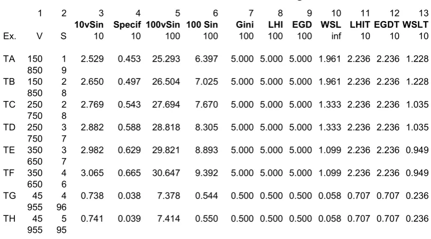
Figure 6 shows how Sin[v, s]^(1 / f) follows from estimated Cos[v, s]. 12 A sensitivity of f = 2 means using √Sin. Looking at some calibrating cases, it appears wise to select the standard value of f = 2 indeed. In Figure 6 the factors 100 and 10 are not included yet.
Figure 6. Sensitivity enhancement with Sin[v, s]1/f = √[1 – Cos[v, s]2] 1/f
Factors 10 or 100 can be introduced to eliminate most leading zeros. Table 5 reviews two cases. With 100, then f = 1 gives the sine values on a scale of 0 to 100. This should not be read as a percentage though. The suggested standard f = 2 takes the square root (keeping the sign) and gives values on a scale of 0 to 10. The latter can be read as an inverted (Bart Simpson) report card. Though the index is straightforward math(s), we likely should not attach great value to the second digit. The use of 10 √Sin seems advisable overall.
Case 1 with large disproportionality is modestly scored as 19.6 by Sin (f = 1) on a scale of
100. Yet f = 2 better conveys the sizeable disproportionality, with a score of 4.4 on a scale of 10, or 44 or a scale of 100.
Case 2 with a small disportionality (that flips the majority) gets –4 on a scale of 100 by
unadjusted Sin, and gets –2 on a scale of 10. The first is unconvincingly insensitive, and thus we may prefer f = 2.
PM 1. The sign indicates the flipping of majority. PM 2. The differences in scales make a design-phase somewhat more complicated. Once the suggested standard f = 2 would be adopted in general, then common comparisons can be on the scale of 10 only, without this potential source of confusion on scale 10 or scale 100.
Table 5. Sensitivity and scale 10 or 100
Votes Seats f = 1 and sign 100 Sin f