Structure and causes of vegetation change in state and transition model applications

(1)

J. Range Manage.

50:39Q-408

Structure and causes of vegetation change in state and transition model applications

RICARDO M. RODRIGUEZ IGLESIAS AND MORT M. KOTEtMANN

Authors are post-doctoral research associate and professor, Department of Rangeland Ecology % Management, Texas A&M University, College Station, Tex. 77843-2126.

Abstract

State and transition (ST) descriptions of rangeland vegetation dynamics provide information on current perceptions of explicit causes of change in dominant vegetation. Structural attributes of ST applications allow an evaluation of the complexity of the ST model and comparisons with the organization of the traditional succession-retrogression model of secondary succession. An analysis of 29 applications of the ST model revealed consistent trends. The number of transitions connecting states showed a less-than+xpected increase with the size of the application. This ls probably associated with limitations to interpret complex I&- tionsbips and a need to produce relatively simple applications.

Larger applications exhibited a shii towards stable states with pivotal positions within structures less co~ected (i.e., with fewer transitions) than expected by chance for a given number of states. Thus, some stable states assume key intermediary roles as the number of states considered increases. It is debatable whether thll is a property of larger systems or an effect of model- ing bii. The analysis of causes of vegetation change conilrmed current perceptions about the importance of man-related sources of disturbance. Grazing, fue, and control of woody piant species are vlsuaiized as the most relevant man-related agents of change.

Some ST applications retain autogenic behaviors embedded in transitions in spite of the event-driven nature of the approach.

However, the ST model removes autogenic procesz~ from their central role as general causes for vegetation change. This approach is theoretically very limited because no general properties or attributes of the components (e.g., plant species assemblages, individual species) or processes (e.g., growth, reproduction, mineralization) of the system are used in any comprehensive way to generate predictive rules of wider than local relevance.

Alternative approaches are suggested that would allow ecological generalizations and comparisons across systems.

Key Words: alternative stable states, climax, fup, grazing, retr+

gression, secondary succession

The senior author acknowledges support received from Texas Agricultural Experiment Station, Consejo National de Investigaciones Cientfficas y T6cnicas (Argentina), Centro de Recursos Naturales Renovables de la Zona Semi6rida (Argentina), and Fundacibn Antorchas (Argentina). The contribution of unpublished material by various authors is gratefully acknowledged. Herman S. Mayeux, Jim C. Noble, and Irnanuel Noy-Meir made helpful suggestions on an earlier version of the manuscript.

Manuscript accepted 14 Aug. 1996.

R&men

Descripciones de la din6mico de la vegetation natural de1 tipo

“estados y transiciones” (ET) proveen information sobre percep ciones actuales acerca de causas explicitas de cambio en vege- tacion dominante. Las caracteristicas estructurales de apllca- ciones de1 modelo ET permiten una evaluation de su complejidad y comparaciones con la organization de1 modelo traditional de sucesion secundaria, basado en secuencias de deterioro-sucesicut.

Un am%isll de 29 aplicaciones del modelo ET revel6 tendencias consistentes.

El increment0 en el nimero de transiciones asociado a un aumento en el numero de e&ados fue menor de1 esperado. Elio se deberia, probablemente, a limitaciones en la interpretscion de rehcioaes complejas y a la necesidad de producir apiicaciones relativamente sencillas. Las aplicaciones de mayor tamaiio tendieron a incluir estados estables centrales inmersos en estruc- turas menos conectadas (i.e. con menos transiciones) que 10 esperable por azar para un cierto numero de e&ados. Ella impli- carla que algunos estados estahles tienden a asumir roles inter- media&s claves en aplicaciones que in&yen un elevado munero de &ados. Es dlscutible que &a sea una propiedad de slstemas extensos o simple sesgo htducido en el uso del modelo.

El anhlisis de causas de cambio en la vegetation confirm6 actuales percepciones acerca de la hnportancia de 10s diiturhios antropog6nico.s. El pastoreo, el uso de1 fuego, y el control de especies legosas aparecen coma 10s mL importantes agentes de cambio antropog6nico. A pesar de ser dinamicamente contro- ledas por even&, algunas aplicaciones de1 mode10 ET conservan elementos autog&ticos. Los procesos autog&icos, sin embargo, aparecen despiazados de su rol central coma causas universales de cambio en la vegetation. El valor te6rico de esta propuesta es muy restrhrgido porque no hate uso de propiedades o atributos de 10s componentes (e.g. especies, grupos de especies) o procesos (e.g. crechniento, reproduction, mineralization) de1 sistema en alguua manera abarcadora que permita formular reglas predic- tivas de aplicacion ampiia. Se sugieren propuestas alternativas que permitirian generalizaciones ecologicas y comparaciones entre diferentes sistemas.

The state and transition (ST) model, named by Westoby et al.

(1989a), has recently become a popular tool for communicating ideas and hypotheses about vegetation change in rangelands. For systems in which it may be meaningful to define ecological objects at a certain scale of perception, the ST model facilitates the capture of relevant system-driving events/processes. It also

(2)

forces the suggestion or indication of explicit causes to justify transitions among states. Although the ST model lacks a spatial component, some of its most recent applications include state- ments about time frame, confidence, and expected probability of transitions (e.g., Ash et al. 1994).

Despite suggestions to the contrary (e.g., Borman and Pyke 1994), the ST model does not represent new ecological theory (Westoby et al. 1989b, Walker 1993). It has been used to describe vegetation dynamics that do not fit within the traditional succession-retrogression (SR) frame of vegetation change in rangelands described by Sampson (1917, 1919) and Dyksterhuis (1949.

1958a, 1958b) and this has probably generated some confusion.

Applications of the ST model are frequently associated with

“community” as opposed to “continuum” theories because of their structure, particularly the splitting of change processes into discrete states when systems are evaluated at pre-selected scales of time and space. This does not necessarily imply support for community-unit ecological theories; rather, it reflects an effort to sim- plify the translation of the supposedly complex operation of ecological objects into understandable diagrams amenable for management decisions. In particular, the dynamics of models presum- ably containing alternative stable states (for a theoretical view, see Law and Morton 1993) are usually depicted using this tool.

This may be justified when the presence of alternative stable states, the occurrence of irreversible changes relative to the selected time scale, or the action of non-linear processes, are hypothesized.

A structural analysis of ST applications may provide an opportunity to evaluate differences and similarities between these

“alternative stable state” schemes and traditional linear (Clements 1916, 1936) or star-like (Dyksterhuis 1949) representations of

“climax-seral stage” models. The explicit implication of particular factors used to explain transitions between states offers a unique opportunity for cataloging and evaluating the relative ire- quency of causes of vegetation change and relationships among such causes. Sources of change of widespread apparent importance can be identified that may be relevant to consider when confronting the task of understanding range dynamics in similar vegetation types-

The objectives of this work were: (1) to identify causes of vegetation change of perceived widespread importance in rangelands, and (2) to assess the potential complexity of the state and transition model through an analysis of 29 applications of this approach. Some structural comparisons with the traditional succession-regression model were possible using regression tech- niques and graphical representations of a stage version of the SR model as the null hypothesis for the ST model.

Materials and Methods

Twenty nine published and unpublished applications of the state and transition model were analyzed (Table 1). Details on unpublished applications are available from the authors upon request. These studies represented the most complete set available and were not subjected to any selective process other than checking for “state and transition” structure and explicit indication of causes of transitions. Some of the studies (Wballey et al.

1978, Wilson et al. 1988, Silcock et al. 1988) predate the publica- tion of the paper that is usually referred to as the original source for the scheme (Westoby et al. 1989a). Most of the models origi-

nated in Australia, with some examples from Argentina, South Africa, Spain, and the US. These applications cover a fairly broad range of rainfall regimes and vegetation types, but most of them were developed for semi-arid grasslands/shrublands.

Clarification of some terms is required to interpret the analyses performed. A state and transition model contains 2 types of objects: stares and transitions. States are physiognomically characterized ecological entities and are usually described by botanical composition of dominant vegetation. Transitions are not always clearly defined and may be classified as simple or complex. Simple transitions involve the action of only 1 possible cause (although it may have more than 1 component; chemical treatment of woody plants and grazing, for example) that may involve 1 or more single factors (e.g., chemical treatment of woody plants, grazing, rainfall, fertilization). Complex transitions may be provoked by more than one cause (grazing or rainfall and summer fire) each of which may involve 1 or more factors. Factors may be additionally characterized by some attribute (e.g., intensity, season) that completes their description.

Complex transitions were distinguished from complex causes (those including more than 1 factor) by means of identifying 3 of the basic connectives of sentential logic in the model descriptions: negation ( 1, i.e., no ). conjunction (A, i.e., and ) and dis- junction ( v, i.e., or ). Stylistic variants of these connectives (e.g., both, although, as well as, unless) were interpreted and translated into 1 of the 3 logic equivalents (Allen and Hand 1992). Some examples follow.

Example 1: transition provoked by summer tire.

1 cause: fire

1 factor: fire (qualified by season) Transition 1: (simple) provoked by factor A

1 cause: A (simple) 1 factor: A

Example 2: transition provoked by no chemical control and no rain and heavy grazing.

Transition 2: (simple) provoked by +A(~B,X)I cause: ~AP.(YBAC) (complex);

3 factors:A, B, and C

Example 3: transition provoked by tire and no grazing or above average rainfall and seeding and no competition.

Transition 3: (complex) provoked by (AA-B) v (G,D,-,yE) 2 causes: A A 7 B (complex) or C A D A 1 E (complex);

Sfactors:A,B,C,D,E

The classification of factors and attributes causing vegetation change required many iterations. The classification developed is obviously not unique.

Causes of Vegetation Change

An analysis of causes of transitions was performed on the set of factors involved as qualified by attributes (a total of 50) and then grouped into 6 main factors determined from this preliminary general classification. Main factors identified were labeled as

grazing, fire, rainfall, woody plant control, other man-related management practices, and endogenous factors. Causes identified as the “absence” or “lack” of single factors (e.g., fire, grazing) or combinations thereof (e.g., rainfall and grazing and no fire) were classified as endogenous based on the rationale that “absence of . . . ” or “lack of . ..‘I . Implied that the system was left to its own spontaneous dynamics involving recruitment of new (possibly woody) plants, aging of perennial species, exhaustion of seed banks, and similar autogenic processes. It is recognized that, in some cases (e.g., purposive fire suppression), this assumption

(3)

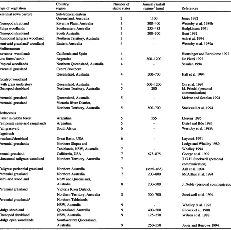
Table 1. Overview of main characteristics of models included in the data base of state and transition applications.

Type of vegetation

country/ ^Number ^of ^Amual ^rainfall

region stable states regime’ (mm) References

Perennial sown pasture Chenopod shrubland Mulga woodlands Chenopod shmbland Monsoonal tallgrass woodland Semi-arid grassland/ woodland MCdite~eil.U

savanna- woodlands LOW forest/ scmb Tropical woodlands Perennial grassland

Eucalypt woodland with grass understory Chenopod shmbland Perennial grassland Perennial grassland

Herbaceous

layer in &d&n forest Temperate semi-arid rangelands Tall grassveld

Sagebrush grassland/shmbland Perennial grasslands Ammal grassland

Monsoonal tallgrass woodland

Tallgrass periennial grassland Perennial grassland Semi-arid woodland

Perennial grassland

Perennial grasslandsz

Mulga shrubland Chenopod shrubland Mulga open woodlands

Sub-tropical eastern Queensland, Australia Riverine Plain, Australia Southeastern Australia South Australia

Northern Territory, Australia Eastern Australia

1100 300-400 253-483 2tXI-300

California and Spain Argentina

Northern Queensland, Australia Central/southern

Queensland, Australia

4 4 4

800-1200

4 500-700 Hall et al. 1994

Queensland, Australia 4 600-1200

Northern Territory, Australia 5 200

Queensland, Australia Victoria River District, Northern Territory, Australia

5

5 500-700 Stockwell et al. 1994

Argentina 5

South Africa 6

555

Great Basin, USA Northern Slopes and Tablelands, NSW, Australia California, USA

Northern Territory, Australia

6

I I 7

675-815

Northern Australia Northern Australia NSW and Queensland, Australia

Victoria River District, Northern Territory, Australia Northern Tablelands, NSW, Australia Queensland, Australia NSW, Australia Southwestern Queensland, Australia

7 (semi-arid)

7 200-800

8 200-500 J. Noble (personal communication)

8 500-700 Stockwell et al. 1994

400-500 125-350

250-550 Jones and Burrows 1994

Jones 1992 Westoby et al. 1989b Hodgkinson 1991 Hunt 1992 Ashet al. 1994 Westoby et al. 1989a

Huntsinger and Bartolome 1992 De Pietri 1992

scan1an 1994

Orr et al. 1994 M. Friedel (personal communication)

M&or and Scanlan 1994

Llorens 1995 Distel and B&J 1995 Westoby et al. 1989b

Laycock 1991

Lodge and Whalley 1989, Whalley 1994

George et al. 1992 T.G.H. Stockwell (personal communication)

Ash et al. 1994 McArthur et al. 1994

Whalley et al. 1978 Silcock et al. 1988 Wilson et al. 1988

‘If indicated in the original documentation.

zModel is an integrated view of 3 different perennial grasslands that were arbitrarily considered as a shole to avoid artificial replication of causes of vegetation change.

might introduce some bias. However, in an overwhelming major- dure allowed us to ascertain relationships between factors that are ity of cases, the correct interpretation was that lack of fire, for frequently cited in association. Results are expressed as occur- example, implied the absence of conditions to apply prescribed rences (i.e., the number of times a particular factor or combina- burning when indicated. References to “climatic conditions” or tion of factors was cited as involved in transitions) and/or fre-

“weather” (a total of 4 instances) were grouped under the “rain- quencies (i.e., occurrences in relation to the total number of

fall-general” label. occurrences and expressed as percentages).

Causes involving 1,2, and 3 or more single factors were classified independently and then pooled to obtain overall estimates of occurrences. A classification was also performed on complex

StnrctU,.al AnalYSis

causes involving exactly 2 or exactly 3 factors. This latter proce- An analysis of some structural attributes of state and transition applications was implemented to study relationships involving

(4)

the number of transitions, the degree of connection among states, and the distribution of transitions among states. Regression tech- niques and graphical representations of null hypotheses were used for these purposes. The rationale for this type of analysis was to evaluate the structural complexity of ST applications relative to a linear or star-like traditional stage-based “succession-retrogression” structure. This rationale requires clarification to avoid possible misinterpretations. Dyksterhuis’ approach to range condition assessment (Dyksterhuis 1949, 1958a, 1958b) is based upon the succession-retrogression (SR) concept, but implemented in the context of a continuum in the vegetation space, i.e., no stages or states are distinguished (Dyksterhuis 1949, 1985). The widespread idea that Dyksterhuis’ condition-relative-to-climax scheme is, somehow, “Clementsian” orthodoxy, is incorrect.

However, and only for the purpose of comparing structural characteristics, SR was represented as linear or star-like sequences of states, more in line with a “traditional” view (e.g., Clements 1916,1936; Sampson 1917,1919).

For the representation of expected values and null hypotheses, the following results were used. The minimum number of transitions (t) required to maintain the integrity of au application with s states is s-l (otherwise at least 1 state will be disconnected from the rest) and corresponds to a linear model (or some topologically equivalent structure) with only one transition linking consecutive states. The maximum number of transitions for an s-sized application of any possible structure is s ( s-l ). Thus, an application with 3 states can have a maximum of up to 6 transitions that will connect each state to the rest through two-way links. The equivalent maximum possible number of transitions for an s-sized application with linear or topologically equivalent structure is 2 ( s-l ).

This is because links are only allowed between contiguous states.

The degree of connectance (c) among states was calculated as the number of indicated transitions (t) relative to the maximum number of possible transitions for a given size, i.e., c = t / ( s ( s-l )), which has a maximum of 1 (when all states are connected through two-way transitions) and a minimum of 1 / s (i.e., when the number of transitions is just enough to keep all states integrated). An estimate of connectance provides a way to evaluate the potential intricacy of the behavior of the system for a given nominal size. The null hypothesis for the expected value of connectance as a function of number of states required the calculation of a probability distribution for every possible number of stable states. For s = 2, the maximum number of possible transitions is 2.

These 2 transitions can be different or the same with the same probability (0.5) only by chance. In the first case, c = l/( 2 ( 2-l ))

= 0.5 while in the second one c = 1.0, so the weighted (connectance values weighted by the probability of occurrence) mean outcome (0.5 x 0.5 + 1.0 x 0.5 ) would be 0.75. The process can be visualized as a random assignment of the maximum number of possible transitions for a given application size (of any possible structure, not necessarily linear) to the possible slots that transitions can occupy among states. A Monte Carlo approach, involving 10 replicates of 20,000 simulations for each nominal size (number of stable states) was used to estimate expected values of

coMectance.

The distribution of transitions, a measure of the concentration or dispersion of transitions among states, was estimated using an ud hoc equitability index (e) derived from Shannon’s information index (Shannon and Weaver 1949):

e=(H-L)/L

where H is Shannon’s index calculated as: H = -ii 1(Pi ln PiI;

s

where pi = $ Et, $ represents transitions as defined above, i is i”’ state and 22 H calculated for a model with completely reversible linear structure, i.e., one in which there would be 2 states (those located at both ends of the linear stntcture) ^connected to the rest by 2 transitions and (s-2 ) other states each cormect- ed by 4 transitions. This equitability index can be used as an indi- cator to detect structural shifts in the distribution of transitions which are indicative of certain states playing key “intermediary”

roles iu the dynamics of the system. Maximum equitabiity will vary with the number of stable states but can be easily calculated from configurations in which each state is connected to every other state by the same number of links, either 1 or 2.

Comparative minimum values of equitability were calculated using the following approach. For each nominal size, all possible configurations of linear and star-like reversible systems were determined and their frequencies and equitabilities calculated tak- ing into account topologically equivalent configurations. A weighted (by frequency) average was then obtained for every possible number of stable states from 3 to 9 (equitabiity is fixed and equal to zero for a 2-state configuration).

Results

The 29 applications contained a total of 162 stable states (Table 1; mean: 5.6 states I application, range: 2-9 ). They provided a total of 310 transitions among states, 369 instances of causes of transitions, and 604 instances of factors involved in causes. In 1.2% of these latter instances (71604 ) the ultimate factor involved was unknown to the author(s) or the corresponding trau-

sition was deemed improbable and the factor involved not identi- tied. Table 2 shows occurrences and relative frequencies of main factors and individual factors within main factors, classified by causes involving one (192), two (264), or three or more (141) single factors. Only individual factors with at least 1.5% of overall frequency are shown in Table 2.

Crazing was the main factor most frequently cited (over 30%

overall relative frequency) although its relative contribution decreased from over 40% to less than 20% as the number of factors involved in causes increased from 1 to 3 or more (Table 2).

Endogenous factors were the second most frequently cited; they approached and finally exceeded the frequency of grazing factors as the number of factors considered increased. Rainfall was the third most frequently cited main factor and showed a trend to increase in relative frequency of citation as the number of factors involved in causes increased. The involvement of fire, woody plant control, and other man-related practices was lower and seemed to be less dependent on the number of factors included in causes although woody plant control increased up to 17% relative frequency when 3 or more factors were considered.

Grazing. A “within main factor” calculation of frequencies for grazing (Table 2) indicated a consistently high relative frequency of citation for intensity of grazing (either alone or interacting with season or system of grazing) that was not associated with the number of factors considered. Trampling, system of grazing, and an interaction factor between system of grazing and animal

(5)

Table 2hiividual and main factors most frequently cited. Values are frequencies (occurrences) classified according to the number of factors involved in causes of transitions.

Main Factor Number of factors involved in causes

Individual factor orazing

by intensity by system x intensity by season x intensity general

by season Endogenous

seedbank absence of fire absence of grazing soil fertility absence of woody plant control Rainfall

ahove average below average general Fire

general by season Woody plant control

chemical mechanical

Other man-related factors seeding

fertilization

One Two Three or more All

43.2 (83) 33.0 (87) 19.9 (28) 33.2 (198)

51.8 (43) 66.7 (58) ^75.0 (21) ^61.6 (122)

18.1 (1% 12.6 (11) 0.0 (0) 13.1 (26)

14.5 (12) ^3.4 ⁽³⁾ ^0.0 ⁽⁰⁾ ^7.6 (15)

7.2 (6) 8.0 (7) 7.1 (2) 7.6 (1%

1.2 (1) 6.9 0% ^10.7 ⁽³⁾ ^5.1 ⁽¹⁰⁾

19.8 (38) 25.4 (67) 24.1 (34) 23.3 (139)

0.0 (0) 32.8 (22) 50.0 (17) 28.1 (39)

26.3 (10) 17.9 (12) ^20.6 (7) 20.9 (29)

23.7 (9) 13.4 (9) 14.7 (5) 16.5 (23)

5.3 (2) ^11.9 63) ^0.0 ⁽⁰⁾ ^7.2 (10)

10.5 (4) 7.5 (5) 0.0 (0) 6.5 (9)

11.5 (22) ^14.0 ⁽³⁷⁾ ^21.3 ⁽³⁰⁾ ^14.9 (8%

27.3 (6) 24.3 (9) 50.0 (15) 33.7 (30)

50.0 (11) 43.2 (16) ^6.7 (2) ^32.6 (29)

9.1 (2) 13.5 (5) 20.0 (6) 14.6 (13)

12.0 (23) 12.9 (34) 12.1 (17) 12.4 (74)

43.5 (10) 61.8 (21) ^88.2 ⁽¹⁵⁾ ^62.2 ⁽⁴⁶⁾

21.7 (5) 8.8 (3) 5.9 (1) 12.2 (9)

6.3 (12) 5.7 (15) 17.0 (24 8.5 (51)

50.0 (6) ^40.0 (6) ^45.8 (11) 45.1 (23)

25.0 (3) 53.3 (8) 50.0 (12) 45.1 (23

7.3 (14) 9.1 04 5.7 (8) 7.7 WI

21.4 (3) 54.2 (13) 62.5 (5) 45.7 (21)

21.4 (3) 29.2 (7) 0.0 (0) 21.7 (10)

Endogenous. The “endogenous” main factor had the largest number and variety of individual factors included. Availability of seed/propagules was the individual factor most frequently referred to within this group although it was never mentioned as the only factor responsible for any transition (Table 2). Other,

less frequently mentioned individual factors were insect out- breaks, absence of various complex causes, establishment of exotics/invaders, competition and absence of competition, plant diseases, increased above ground primary production, plant dieback, soil surface conditions, and absence of cultivation. The absence of a factor (e.g., no fire, no grazing) was the most frequently invoked cause of change within this group, accounting for over 50% (72/139) of all instances. When this uninformative composite factor was removed from calculations, the frequency of citation of seed bank status increased to 54.2% ( 39 / 72 ) with similar incidences when 2 ( 22 / 41) or 3 or more ( 17 / 22 ) individual factors were considered.

Rainfall and Fire. These main factors were cited a similar ntmt- ber of times (Table 2) although the internal distribution within main factors was remarkably different. Most frequent references involving rainfall mentioned lack of rain (or drought) and above average precipitation (or some stylistic variants) with rainfall as a general event mentioned less frequently (Table 2). Also, opposite trends with the number of individual factors involved were observed for above and below average precipitation. Season, timing of ram, timing of ram interacting with amount of rainfall, and season interacting with amount of rainfall accounted for the rest of the occurrences within this main factor.

Fire was rarely qualified as dependent on the usual attributes of season, frequency, and intensity (Table 2) and interactions

between those attributes were only mentioned in 3 instances of fue involvement. Wildfiis or wildfire control, intensity of fire, and an interaction between frequency and intensity of fire complete the list of individual fire-related factors.

Woody Plant Control and Other Man-related Factors. Patterns of relative frequency within the “woody plant control” and “other”

groups are probably much less reliable because of the reduced number of instances involved. Nevertheless, similar frequencies of chemical and mechanical control of woody plants were observed (Table 2), with biological control and plant control as a general factor, less frequently considered. Man-related factors other than those indicated in Table 2 were overharvest of propagules, soil reclamation, cultivation, and weeding.

Pairs of Factors. Main factors most frequently mentioned together included grazing and endogenous factors, grazing and fire, and grazing and rainfall (Table 3). Marginal frequencies (last column in Table 3) differ slightly from the distribution of two- factor causes in Table 2 because contributions from pairs consti- tuted by the same factor count double in Table 3. Results from the occurrence of three-factor causes (117 instances) followed similar trends with grazing, rainfall, and endogenous as the most important groups of factors (59.0,56.4, and 51.3%, respectively), followed by woody plant control (46.1%), fire (38.5%). and other man-related practices (12.8%).

Frequency of main factors varied among applications, and for those with 3 or more states, there was no apparent pattern of change associated with the number of states (Fig. 1). Frequency of endogenous factors tended to follow an inverse trend relative to grazing factors. Rainfall and grazing were the only factors mentioned in the 2-state application included in the analysis (Fig. 1).

(6)

Tahk3.-(~ddlUereatprdndectonu-d~W *=d-- en,tl=h

~rmavplnntm=~oHpc),~~ mawdakdnnblfectorkLlek.

Grazing Endosewus Fm Rainfall oom (man) lwc Ovedl ,

Requsncy

-g 1 (0.8) 34 (25.8) 22 (16.lJ 20(15.1) 2 (1.5) l(5.3) 65.1

we== 11 (8.3) 3 (2.3) 7 (5.3) 1 (0.8) 0 (0.0) 42.4

Fm 0 (0.0) 4 (3.0) 0 (0.0) 5 (3.8) 25.8

Rainfall 2 (1.3 2 (1.5) 0 (0.0) 26.5

-(man) 8 (6.1) 3 (2.3) 12.1

WPC 0 (0.0) 11.4

‘Luacolmlmsbo*saarmnU~M -dsrh*-~vcm*~-c4*~t32~.

Structuml Analysis

Results tium s4nwlwal analysea ate summarized in Figs. 2 to 4.

As expected, tbe number of transitions increased with the number of states although 2 of the applications only exhibited enough transitions to exactly keep the integrity corresponding to their nominal size (Fig. 2). A linear regzzssioo of nuntbcr of h-aasitioas against numtm of statos in log-log scale was found to adequately desclibe this relationship ( P < 0.001 , r = 0.73 ) and attenuated an increase in variance associated with the number of states. Non- linear alkmativea did not improve this fit significantly. The slope of this relationship in the linear scale ( 1.82 * 0.322 ; b * SE ) was compared to the expected value for applications with linear or topologicaUy equivalent structure (i.e., 2) sod found not significantly dikent (t = 0.56; 27 d.f.). The theoretical iotemept (i.e..

-2) was within the standard error of the calculated intercept (0.W f 1.921) and coaseqaently not signiricaatly different ftom it (t = 1.06; 27 d.f.). Points corresponding to applications with minimum numbers of transitions for their nominal size (Fig. 2) showed up as potential outliers in many diagnostic plots. eveo in log-log scale. Removing those data. however, did oot change any result so they were retained.

Average coonectaace among states tended to deaease with an increase in the number of states (pig. 3). Average cooncctancc was close to theoretical expected values for applications with few states but declined, approaching minimum conoectance, as the

NUMBER OF STATES Fig.1.Rdativefrequencieaofmainfwtnrs~htnnsitbara3

a fmwtien of the numbv of stable states.

number of states incraasod. The equitability index (Fig. 4) showed similar behavior. Applications with 4 or fewer stable states exhibited null or positive deviations (i.e., more uniform distribution of linlcs than with a Iii or topologically eqoivaleot reveraihle structure) except for 1 case, while applications with 5 or more statea showed increasingly negative deviations.

Although the set of state and traosition applications analyzed does not represent any particular ecological system or region.

sane. general shuctural features cao be charaderized and applied for developing other applicatioos. The relative fiqoaocy of factors cited as causea of vegetation change in this cokction of ST applications does not neccssatily apply in general to rangelaods.

but does reflect cumnt main-stream range management ideas (Stafford Smith and Pickup 1993). The high relative tirqoencies with which certain factors and groups of factors were cited is a

loo,- 1

1

2 9

NUMBER OF STATES mg.20bseRItbasodaeksymbDk)andapectedrelatbnship(rolid

he) descrtbtng the number of transitiona w a hodion of the nnmher of stabk statea under the pssumptka of linear (or tape logkally equivalent) structure. Dotted ltnes indtate allownbk maxims and minims for the observatkaa Clumped obswvattona

@nunher of states 3,4,5, and ll wem jittered by adding random noke to improve vtsunlivtioa

(7)

y 0.6 2 5 0.4 z 5 0 0.2

a

NUMBER OF STATES

Fii. 3. Observed (black symbols) and expected (solid line) values for connectance. Maximum and minimum values allowable are buli- cated by the dotted lines. Clumped observations (number of states 3,4,5, and 7) were jittered by adding random noise to improve visualization.

consequence of their perceived widespread importance across a variety of rangeland types (see Fig. 1). In this sense, sources of change frequently mentioned in these applications should be considered when evaluating the dynamics of similar types of rangelands.

Among the factors that can be controlled by management, intensity of grazing is obviously considered the most important single cause of vegetation change followed by the use of fire.

Other management practices like chemical or mechanical woody plant control and seeding account for a much reduced relative frequency of citation. However, when considered as a whole, man- related factors justify more than 60% (364/597) of the total number of instances of identified factors, Rainfall (15%) and endogenous factors (23%) account for the rest. Although this partition depends on a non-unique classification of individual factors, it is surprising that about 20% (38/192) of simple instances of transitions and 23% of the total were attributed to the action of auto- genie factors. This is hardly expected for system components that are supposed to remain relatively stable when external forces are not operating (Laycock 1991). Some of the endogenous “factors”

cited (e.g., availability of propagules) may well be considered conditions required for the operation of other factors, rather than genuine and ultimate causes of change. However, almost half (68/139) of the instances included in the “endogenous” group of factors corresponded to cases of “absence of . ..‘I. particularly of grazing or tire. This is a clear indication that certain spontaneous behavior still remains embedded in the structure of some ST applications, even if not explicitly modeled.

Two trends were observed relative to the number of factors considered. The overwhelming frequency of citation of grazing when only single factors are considered was moderated by an

increasing relevance of factors such as seed bank dynamics (Table 2) up to a point in which grazing was no longer the most frequently cited main factor. Above and below average rainfall regimes exhibited opposite trends associated with the number of factors considered (Table 2). This probably reflects the fact that droughts can severely modify the botanical composition of a site by themselves while a good rain needs to be accompanied by other factors or conditions, like availability of propagules or a reduction of stocking rate, to produce similar effects.

The analysis of pairs of factors (Table 3) was in general agree- ment with the trends discussed above. Additive, interactive or sequential effects involving grazing seem to be the most common instances of complex factors.

Structural Analysis

The structural analyses revealed an economy of transitions between states remarkably similar to what would be expected for linear or star-like succession-retrogression models of comparable dimensions (Fig. 2). Accordingly, the likelihood of transition from a given state towards any other possible state was propor-

tionally lower for larger state and transition applications (Fig. 3).

A similar phenomenon is usually observed in ecological webs (Yodzis 1980, Warren 1994), although in this latter case it may well be due to defective sampling. In our case, the observed decrease in connectance may indicate a real trend associated with an increase in the complexity of the applications. Alternatively, and more probably, it reflects human limitations to visualize complex systems. The decrease in connectance was associated with a shift in the distribution of transitions (Fig. 4) from applications with states more evenly connected than expected for a reversible linear structure towards applications with a more biased distribution of transitions among states. This indicates that some stable states tend to assume central or key roles as the number of states considered increases. With climax removed from its central role as the reference state in succession-deterioration sequences, more equitability among states would be expected. A

*- =! 04,

f$ L. .

a I,

8 -2 .*- f-.

.

*.__

---..,

..-.__._ . 1

4 . . .-.-...,_

. .~~..._____.__

-6l I I 9 .

3 i

4 5 6 7 8 9

NUMBER OF STATES

Fii. 4. Observed values for the equitability index as a function of the number of stable states. Maximum and minimum values allowable for Linear or topologically equivalent structures are indicated by dotted lines. Clumped observations (number of states 3,4, and 5) were jittered by adding random noise to improve visualization.

(8)

possible explanation is that those central intermediary states are the best known or the ones most frequently observed under current management conditions. Familiarity with a certain common state of the vegetation may bias the general picture of the system.

Again, it is difficult to ascertain to what extent a decreased equitability is a real property of larger systems or simply an effect of the way human minds look at the world. Some of the structural properties observed may be more related to the psychology of perception than to any real characteristic of increasingly complex systems.

Two striking outcomes from these analyses are the elementary nature of causes of change and the structural simplicity of the applications. More than half of the instances of transitions for which some explanation was provided involved only 1 factor (206/359), possibly modified by the attachment of some attribute.

In 90% of the instances (324/359), transitions were associated with at most 2 factors. In only 2% of the cases were transitions justified by the action of complex causes involving 4 factors. In addition, wording of complex causes involving 2 or more factors generally corresponded to a mental image of additivity or sequential effects rather than of interactions among factors. This is in sharp contrast with the generally acknowledged complexity of vegetation dynamics (Roberts 1987, Wiegleb 1989) and reveals the equivalent of a statistical “main effects” linear model operating at each node (stable state) in state and transition applications.

The reasonableness of this approach may well be justified in the necessity of providing unsophisticated management-level predic- tions and/or in the lack of a consistent ecological theory about the spontaneous behavior of complex ecological objects.

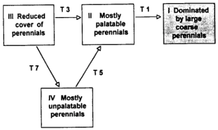
The dynamic represented in Fig. 5 is a good example of how spontaneous and “external” causes of change are weighted in ST applications. Fig. 5 is a modification of Fig. 5 from Westoby et al. (1989b) in which all man-related causes of change have been removed. According to what is left from the original ST application, in a hands-off scenario and given enough time, the system would tend to reach a unique stable state that would persist unless the system were put under some disturbance stress. Many ST applications can be reduced to similar schemes by means of removing identifiable “non-spontaneous” causes of change. What is usually left, in turn, is very similar to traditional succession schemes in which a certain sequence of seral stages, terminating in a unique stable state, was hypothesized to represent the sponta-

Fig. 5. ST application from Westoby et al. (1989$ Fii. S), modiied by removing transitions provoked by man-related causes of vegetation change.

neous behavior of the system when freed from disturbances.

Thus, compared to traditional seral stages-climax ideas, the ST approach shifts the relative importance of causes of change by means of overweighing identifiable man-caused factors and down- playing autogenic factors like modifications of soil properties and competition. In doing this, however, the power of an all-encom- passing theory of ecological system behavior is lost and replaced by ad hoc local shifts that fit previously observed vegetation changes under the influence of local prevailing disturbance forces.

This may be realistic, but it is also theoretically very limited because no general properties or attributes of the components (e.g., plant species assemblages, individual species) or processes (e.g., growth, reproduction, mineralization) of the system are used in any general way to generate prediction rules of wider than local relevance. The cohesive nature contributed by processes involved in autogenic succession is removed from its central role of providing a coherent general reason for vegetation change but no alternative comprehensive properties are invoked to fill the gap.

The closest thing to a theoretical support for favoring state and transition representations of ecological systems is provided by the hypothesized existence of alternative stable states in those systems (Lewontin 1969, Sutherland 1974). A thorough discussion of this subject is out of the scope of the present paper but a brief comment on it is worthwhile. The existence of alternative stable states in very simple mathematical systems (see, for example, Noy-Meir 1975) has been widely invoked as evidence favoring the possible occurrence of alternative stable states in complex ecological systems (see, for example, Scheffer et al. 1993). This is a misleading assumption. No general principle can be invoked to justify any similarity between the behavior of a closed isolated mathematical system and the functioning of an open real complex adaptive system with diffuse boundaries. There is no evident reason to assume that more complex entities than those usually represented by Lotka-Volterra equations or similar predator-prey dynamics would behave in a similar way. In fact, empirical evidence frequently shows that the opposite may be true due to com- pensating effects induced by interactions with other systems within a common local landscape. Thus, general equilibrium conditions may emerge asymptotically at certain spatial scales

(DeAngelis and Waterhouse 1987).

The correct interpretation of Noy-Meir’s graphical exercise (Noy-Meir 1975) is that simplicity does not preclude the possible existence of alternative stable states in grazing systems if the assumptions and strong simplifications embedded in the mathematical abstraction are tenable. However, what is a “state” and what is “stable” depends primarily on our perception of change;

i.e., on the temporal and spatial scale at which abstractions of real- ity are being produced. In this sense, it may be fruitful to dissect a system’s behavior into discrete states, if looking at its functioning at such a scale facilitates interpretation and management decisions. This procedure does not require theoretical justification.

Producing theoretical support in the form of unifying ecological principles with predictive capability, based upon the concept of discrete states, is a different, yet unsolved problem (Stafford Smith 1992). Some examples of possibly alternative stable states have been reported in various ecosystems (Barkai and McQuaid 1988, Dublin et al., 1990, Scheffer et al. 1993) but the question still remains whether the nature of those states is dependent upon the intrinsic dynamic of the ecological objects or, in contrast, whether they are produced by some “external” forces alien to the