Adaptive Joint Learning of Compositional and Non Compositional Phrase Embeddings

Adaptive Joint Learning of

Compositional and Non-Compositional Phrase Embeddings

Kazuma Hashimoto and Yoshimasa Tsuruoka

The University of Tokyo, 3-7-1 Hongo, Bunkyo-ku, Tokyo, Japan {hassy,tsuruoka}@logos.t.u-tokyo.ac.jp

Abstract

We present a novel method for jointly learning compositional and non-compositional phrase embeddings by adaptively weighting both types of em-beddings using a compositionality scoring function. The scoring function is used to quantify the level of compositionality of each phrase, and the parameters of the function are jointly optimized with the ob-jective for learning phrase embeddings. In experiments, we apply the adaptive joint learning method to the task of learning embeddings of transitive verb phrases, and show that the compositionality scores have strong correlation with human ratings for verb-object compositionality, substantially outperforming the previous state of the art. Moreover, our embeddings improve upon the previous best model on a transitive verb disambiguation task. We also show that a simple ensemble technique further improves the results for both tasks.

1 Introduction

Representing words and phrases in a vector space has proven effective in a variety of language pro-cessing tasks (Pham et al., 2015; Sutskever et al., 2014). In most of the previous work, phrase em-beddings are computed from word emem-beddings by using various kinds of composition functions. Such composed embeddings are called composi-tional embeddings. An alternative way of comput-ing phrase embeddcomput-ings is to treat phrases as scomput-ingle units and assigning a unique embedding to each candidate phrase (Mikolov et al., 2013; Yazdani et al., 2015). Such embeddings are called non-compositional embeddings.

Relying solely on non-compositional embed-dings has the obvious problem of data sparsity (i.e. rare or unknown phrase problems). At the same time, however, using compositional embeddings is not always the best option since some phrases are inherently non-compositional. For example, the phrase “bear fruits” means “to yield results”1 but it is hard to infer its meaning by composing the meanings of “bear” and “fruit”. Treating all phrases as compositional also has a negative ef-fect in learning the composition function because the words in those idiomatic phrases are not just uninformative but can serve as noisy samples in the training. These problems have motivated us to adaptively combine both types of embeddings.

Most of the existing methods for learning phrase embeddings can be divided into two ap-proaches. One approach is to learn compositional embeddings by regarding all phrases as composi-tional (Pham et al., 2015; Socher et al., 2012). The other approach is to learn both types of embed-dings separately and use the better ones (Kartsak-lis et al., 2014; Muraoka et al., 2014). Kartsak(Kartsak-lis et al. (2014) show that non-compositional embed-dings are better suited for a phrase similarity task, whereas Muraoka et al. (2014) report the opposite results on other tasks. These results suggest that we should not stick to either of the two types of embeddings unconditionally and could learn better phrase embeddings by considering the composi-tionality levels of the individual phrases in a more flexible fashion.

In this paper, we propose a method that jointly learns compositional and non-compositional em-beddings by adaptively weighting both types of phrase embeddings using a compositionality scor-ing function. The scorscor-ing function is used to quan-tify the level of compositionality of each phrase

1_{The definition is found at http://idioms.}

thefreedictionary.com/bear+fruit.

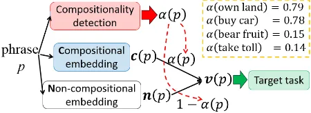
Figure 1: The overview of our method and ex-amples of the compositionality scores. Given a phrasep, our method first computes the composi-tionality scoreα(p) (Eq. (3)), and then computes the phrase embedding v(p) using the composi-tional and non-composicomposi-tional embeddings, c(p) andn(p), respectively (Eq. (2)).

and learned in conjunction with the target task for learning phrase embeddings. In experiments, we apply our method to the task of learning transitive verb phrase embeddings and demonstrate that it allows us to achieve state-of-the-art performance on standard datasets for compositionality detec-tion and verb disambiguadetec-tion.

2 Method

In this section, we describe our approach in the most general form, without specifying the func-tion to compute the composifunc-tional embeddings or the target task for optimizing the embeddings.

Figure 1 shows the overview of our proposed method. At each iteration of the training (i.e. gradient calculation) of a certain target task (e.g. language modeling or sentiment analysis), our method first computes a compositionality score for each phrase. Then the score is used to weight the compositional and non-compositional embed-dings of the phrase in order to compute the ex-pected embedding of the phrase which is to be used in the target task. Some examples of the com-positionality scores are also shown in the figure. 2.1 Compositional Phrase Embeddings The compositional embedding c(p) ∈ Rd×1 _{of a} phrasep= (w1,· · · , wL)is formulated as

c(p) =f(v(w1),· · · ,v(wL)), (1)

where d is the dimensionality, L is the phrase length, v(·) ∈ Rd×1 _{is a word embedding, and} f(·) is a composition function. The function can be simple ones such as element-wise addi-tion or multiplicaaddi-tion (Mitchell and Lapata, 2008).

More complex ones such as recurrent neural net-works (Sutskever et al., 2014) are also commonly used. The word embeddings and the composi-tion funccomposi-tion are jointly learned on a certain target task. Since compositional embeddings are built on word-level (i.e. unigram) information, they are less prone to the data sparseness problem.

2.2 Non-Compositional Phrase Embeddings In contrast to the compositional embedding, the non-compositional embedding of a phrasen(p)∈

Rd×1 _{is independently parameterized, i.e., the} phrasepis treated just like a single word. Mikolov et al. (2013) show that non-compositional em-beddings are preferable when dealing with id-iomatic phrases. Some recent studies (Kartsak-lis et al., 2014; Muraoka et al., 2014) have dis-cussed the (dis)advantages of using compositional or non-compositional embeddings. However, in most cases, a phrase is neither completely com-positional nor completely non-comcom-positional. To the best of our knowledge, there is no method that allows us to jointly learn both types of phrase em-beddings by incorporating the levels of composi-tionality of the phrases as real-valued scores. 2.3 Adaptive Joint Learning

To simultaneously consider both compositional and non-compositional aspects of each phrase, we compute a phrase embeddingv(p) by adaptively weightingc(p)andn(p)as follows:

v(p) =α(p)c(p) + (1−α(p))n(p), (2) where α(·) is a scoring function that quantifies the compositionality levels, and outputs a real value ranging from 0 to 1. What we expect from the scoring function is that large scores indicate high levels of compositionality. In other words, when α(p) is close to 1, the compositional em-bedding is mainly considered, and vice versa. For example, we expect α(buy car) to be large and α(bear fruit)to be small as shown in Figure 1.

We parameterize the scoring function α(p) as logistic regression:

Updating the model parameters Given the par-tial derivative δp = _∂v∂J(p) ∈ Rd×1 for the target

task, we can compute the partial derivative for up-datingW as follows:

δα =α(p)(1−α(p)){δp·(c(p)−n(p))} (4)

∂J

∂W =δαφ(p). (5)

Ifφ(p)is not constructed by static features but is computed by a feature learning model such as neu-ral networks, we can propagate the error termδα

into the feature learning model by the following equation:

∂J

∂φ(p) =δαW. (6) When we use only static features, as in this work, we can simply compute the partial derivatives ofJ with respect toc(p)andn(p)as follows:

∂J

∂c(p) =α(p)δp (7) ∂J

∂n(p) = (1−α(p))δp. (8) As mentioned above, Eq. (7) and (8) show that the non-compositional embeddings are mainly up-dated when α(p) is close to 0, and vice versa. The partial derivative _∂∂J_c(p) is used to update the model parameters in the composition function via the backpropagation algorithm. Any differentiable composition functions can be used in our method. Expected behavior of our method The training of our method depends on the target task; that is, the model parameters are updated so as to mini-mize the cost function as described above. More concretely,α(p)for each phrasepis adaptively ad-justed so that the corresponding parameter updates contribute to minimizing the cost function. As a result, different phrases will have different α(p) values depending on their compositionality. If the size of the training data were almost infinitely large, α(p) for all phrases would become nearly zero, and the non-compositional embeddingsn(p) are dominantly used (since that would allow the model to better fit the data). In reality, however, the amount of the training data is limited, and thus the compositional embeddingsc(p)are effectively used to overcome the data sparseness problem. 3 Learning Verb Phrase Embeddings This section describes a particular instantiation of our approach presented in the previous section,

fo-cusing on the task of learning the embeddings of transitive verb phrases.

3.1 Word and Phrase Prediction in Predicate-Argument Relations

Acquisition of selectional preference using em-beddings has been widely studied, where word and/or phrase embeddings are learned based on syntactic links (Bansal et al., 2014; Hashimoto and Tsuruoka, 2015; Levy and Goldberg, 2014; Van de Cruys, 2014). As with language modeling, these methods perform word (or phrase) prediction us-ing (syntactic) contexts.

In this work, we focus on verb-object rela-tionships and employ a phrase embedding learn-ing method presented in Hashimoto and Tsuruoka (2015). The task is a plausibility judgment task for predicate-argument tuples. They extracted Subject-Verb-Object (SVO) and SVO-Preposition-Noun (SVOPN) tuples using a probabilistic HPSG parser, Enju (Miyao and Tsujii, 2008), from the training corpora. Transitive verbs and preposi-tions are extracted as predicates with two argu-ments. For example, the extracted tuples include (S, V, O) = (“importer”, “make”, “payment”) and (SVO, P, N) = (“importer make payment”, “in”, “currency”). The task is to discriminate between observed and unobserved tuples, such as the (S, V, O) tuple mentioned above and (S, V’, O) = (“im-porter”, “eat”, “payment”), which is generated by replacing “make” with “eat”. The (S, V’, O) tuple is unlikely to be observed.

For each tuple(p, a1, a2)observed in the train-ing data, a cost function is defined as follows:

−logσ(s(p, a1, a2))−logσ(−s(p0, a1, a2))

−logσ(−s(p, a0₁, a2))

−logσ(−s(p, a1, a02)), (9)

where s(·) is a plausibility scoring function, and p,a1 anda2 are a predicate and its arguments, re-spectively. Each of the three unobserved tuples (p0_{, a}

1, a2), (p, a01, a2), and (p, a1, a02) is gener-ated by replacing one of the entries with a random sample.

In their method, each predicatepis represented with a matrixM(p) ∈ Rd×d _{and each argument}

awith an embedding v(a) ∈ Rd×1_{. The} matri-ces and embeddings are learned by minimizing the cost function usingAdaGrad(Duchi et al., 2011). The scoring function is parameterized as

and the VO and SVO embeddings are computed as

v(V O) =M(V)v(O) (11)

v(SV O) =v(S)v(V O), (12)

as proposed by Kartsaklis et al. (2012). The op-eratordenotes element-wise multiplication. In summary, the scores are computed as

s(V, S, O) =v(S)·v(V O) (13) s(P, SV O, N) =v(SV O)·(M(P)v(N)).

(14)

With this method, the word and composed phrase embeddings are jointly learned based on co-occurrence statistics of predicate-argument struc-tures. Using the learned embeddings, they achieved state-of-the-art accuracy on a transi-tive verb disambiguation task (Grefenstette and Sadrzadeh, 2011).

3.2 Applying the Adaptive Joint Learning In this section, we apply our adaptive joint learn-ing method to the task described in Section 3.1. We here redefine the computation of v(V O) by first replacingv(V O)in Eq. (11) withc(V O)as,

c(V O) =M(V)v(O), (15)

and then assigningV Otopin Eq. (2) and (3):

v(V O) =α(V O)c(V O) + (1−α(V O))n(V O), (16) α(V O) =σ(W ·φ(V O)). (17)

The v(V O) in Eq. (16) is used in Eq. (12) and (13). We assume that the candidates of the phrases are given in advance. For the phrases not included in the candidates, we setv(V O) = c(V O). This is analogous to the way a human guesses the meaning of an idiomatic phrase she does not know. We should note thatφ(V O)can be computed for phrases not included in the candidates, using par-tial features among the features described below. If any features do not fire, φ(V O) becomes 0.5 according to the logistic function.

For the feature vectorφ(V O), we use the fol-lowing simple binary and real-valued features:

• indices of V, O, and VO

• frequency and Pointwise Mutual Information (PMI) values of VO.

More concretely, the first set of the features (in-dices of V, O, and VO) is the concatenation of traditional one-hot vectors. The second set of features, frequency and PMI (Church and Hanks, 1990) features, have proven effective in detect-ing the compositionality of transitive verbs in Mc-Carthy et al. (2007) and Venkatapathy and Joshi (2005). Given the training corpus, the frequency feature for a VO pair is computed as

freq(V O) = log(count(V O)), (18) wherecount(V O)counts how many times the VO pair appears in the training corpus, and the PMI feature is computed as

PMI(V O) = logcount(V O)count(∗)

count(V)count(O) , (19) wherecount(V),count(O), andcount(∗)are the counts of the verb V, the object O, and all VO pairs in the training corpus, respectively. We nor-malize the frequency and PMI features so that their maximum absolute value becomes 1.

4 Experimental Settings 4.1 Training Data

As the training data, we used two datasets, one small and one large: the British National Corpus (BNC) (Leech, 1992) and the English Wikipedia. More concretely, we used the publicly available data2 _{preprocessed by Hashimoto and Tsuruoka} (2015). The BNC data consists of 1.38 million SVO tuples and 0.93 million SVOPN tuples. The Wikipedia data consists of 23.6 million SVO tu-ples and 17.3 million SVOPN tutu-ples. Follow-ing the provided code3_{, we used exactly the same} train/development/test split (0.8/0.1/0.1) for train-ing the overall model. As the third traintrain-ing data, we also used the concatenation of the two data, which is hereafter referred to asBNC-Wikipedia.

We applied our adaptive joint learning method to verb-object phrases observed more than K times in each corpus. K was set to 10 for the BNC data and 100 for the Wikipedia and BNC-Wikipedia data. Consequently, the non-compositional embeddings were assigned to 17,817, 28,933, and 30,682 verb-object phrase types in the BNC, Wikipedia, and BNC-Wikipedia data, respectively.

2_{http://www.logos.t.u-tokyo.ac.jp/}

˜hassy/publications/cvsc2015/

3_{https://github.com/hassyGo/}

4.2 Training Details

The model parameters consist of d-dimensional word embeddings for nouns, non-compositional phrase embeddings, d×d-dimensional matrices for verbs and prepositions, and a weight vector

W for α(V O). All the model parameters are jointly optimized. We initialized the embeddings and matrices with zero-mean gaussian random val-ues with a variance of 1

d and d12, respectively, and W with zeros. InitializingW with zeros forces the initial value of eachα(V O)to be0.5since we use the logistic function to computeα(V O).

The optimization was performed via mini-batch AdaGrad (Duchi et al., 2011). We fixed d to 25 and the mini-batch size to 100. We set candidate values for the learn-ing rate ε to {0.01,0.02,0.03,0.04,0.05}. For the weight vector W, we employed L2-norm regularization and set the coefficient λ to {10−3_,10−4_,10−5_,10−6_{,0}. For selecting} the hyperparameters, each training process was stopped when the evaluation score on the devel-opment split decreased. Then the best perform-ing hyperparameters were selected for each train-ing dataset. Consequently, ε was set to0.05 for all training datasets, andλwas set to10−6_,10−3_, and 10−5 _{for the BNC, Wikipedia, and} BNC-Wikipedia data, respectively. Once the training is finished, we can use the learned embeddings and the scoring function in downstream target tasks.

5 Evaluation on the Compositionality Detection Function

5.1 Evaluation Settings

Datasets First, we evaluated the learned com-positionality detection function on two datasets, VJ’054 _{and MC’07}5_{, provided by Venkatapathy} and Joshi (2005) and McCarthy et al. (2007), respectively. VJ’05 consists of 765 verb-object pairs with human ratings for the compositional-ity. MC’07 is a subset of VJ’05 and consists of 638 verb-object pairs. For example, the rating of “buy car” is 6, which is the highest score, indicat-ing the phrase is highly compositional. The ratindicat-ing of “bear fruit ” is 1, which is the lowest score, in-dicating the phrase is highly non-compositional.

4_{http://www.dianamccarthy.co.uk/}

downloads/SVAJ2005compositionality_ rating.txt

5_{http://www.dianamccarthy.co.uk/}

downloads/emnlp2007data.txt

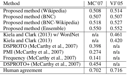
Method MC’07 VJ’05

Proposed method (Wikipedia) 0.508 0.514 Proposed method (BNC) 0.507 0.507 Proposed method (BNC-Wikipedia) 0.518 0.527 Proposed method (Ensemble) 0.550 0.552 Kiela and Clark (2013) w/ WordNet n/a 0.461 Kiela and Clark (2013) n/a 0.420 DSPROTO (McCarthy et al., 2007) 0.398 n/a PMI (McCarthy et al., 2007) 0.274 n/a Frequency (McCarthy et al., 2007) 0.141 n/a DSPROTO+ (McCarthy et al., 2007) 0.454 n/a

Human agreement 0.702 0.716

Table 1: Compositionality detection task.

Evaluation metric The evaluation was per-formed by calculating Spearman’s rank correlation scores6 _{between the averaged human ratings and} the learned compositionality scoresα(V O). Ensemble technique We also produced the re-sult by employing an ensembletechnique. More concretely, we used the averaged compositionality scores from the results of the BNC and Wikipedia data for the ensemble result.

5.2 Results and Discussion 5.2.1 Result Overview

Table 1 shows our results and the state of the art. Our method outperforms the previous state of the art in all settings. The result denoted as Ensem-ble is the one that employs the ensemble tech-nique, and achieves the strongest correlation with the human-annotated datasets. Even without the ensemble technique, our method performs better than all of the previous methods.

Kiela and Clark (2013) used window-based co-occurrence vectors and improved their score us-ing WordNet hypernyms. By contrast, our method does not rely on such external resources, and only needs parsed corpora. We should note that Kiela and Clark (2013) reported that their score did not improve when using parsed corpora. Our method also outperforms DSPROTO+, which used a small amount of the labeled data, while our method is fully unsupervised.

We calculated confidence intervals (P < 0.05) using bootstrap resampling (Noreen, 1989). For example, for the results using the BNC-Wikipedia data, the intervals on MC’07 and VJ’05 are (0.455, 0.574) and (0.475, 0.579), respectively. These re-sults show that our method significantly outper-forms the previous state-of-the-art results.

Phrase Gold standard (a) BNC (b) Wikipedia BNC-Wikipedia Ensemble ((a)+(b))×0.5

(A)

buy car 6 0.78 0.71 0.80 0.74

own land 6 0.79 0.73 0.76 0.76

take toll 1.5 0.14 0.11 0.06 0.13

shed light 1 0.21 0.07 0.07 0.14

bear fruit 1 0.15 0.19 0.17 0.17

(B) make noise_{have reason} 6₅ 0.37_0.26 0.33_0.39 0.30_0.33 0.35_0.33 (C) smoke cigarette_{catch eye} 6₁ 0.56_0.48 0.90_0.14 0.78_0.17 0.73_0.31

Table 2: Examples of the compositionality scores.

Figure 2: Trends ofα(V O)during the training on the BNC data.

5.2.2 Analysis of Compositionality Scores Figure 2 shows howα(V O)changes for the seven phrases during the training on the BNC data. As shown in the figure, starting from0.5,α(V O)for each phrase converges to its corresponding value. The differences in the trends indicate that our method can adaptively learn compositionality lev-els for the phrases. Table 2 shows the learned com-positionality scores for the three groups of the ex-amples along with the gold-standard scores given by the annotators. The group (A) is considered to be consistent with the gold-standard scores, the group (B) is not, and the group (C) shows exam-ples for which the difference between the compo-sitionality scores of our results is large.

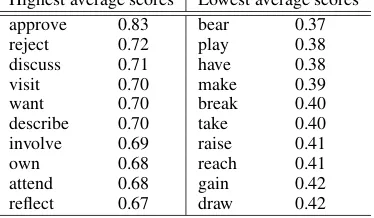
Characteristics of light verbs The verbs “take”, “make”, and “have” are known as light verbs 7_{, and the scoring function tends to assign} low scores to light verbs. In other words, our

7_{In Section 5.2.2 in Newton (2006), the termlight verbis} used to refer to verbs which can be used in combination with some other element where their contribution to the meaning of the whole construction is reduced in some way.

Highest average scores Lowest average scores

approve 0.83 bear 0.37

reject 0.72 play 0.38

discuss 0.71 have 0.38

visit 0.70 make 0.39

want 0.70 break 0.40

describe 0.70 take 0.40 involve 0.69 raise 0.41

own 0.68 reach 0.41

attend 0.68 gain 0.42

reflect 0.67 draw 0.42

Table 3: The 10 highest and lowest average com-positionality scores with the corresponding verbs on the BNC data.

method can recognize that the light verbs are frequently used to form idiomatic (i.e. non-compositional) phrases. To verify the assumption, we calculated the average compositionality score for each verb by averaging the compositionality scores paired with its candidate objects. Here we used 135 verbs which take more than 30 types of objects in the BNC data. Table 3 shows the 10 highest and lowest average scores with the corre-sponding verbs. We see that relatively low scores are assigned to the light verbs as well as other verbs which often form idiomatic phrases. As shown in the group (B) in Table 2, however, light verb phrases are not always non-compositional. Despite this, the learned function assigns low scores to compositional phrases formed by the light verbs. These results suggest that using a more flexible scoring function may further strengthen our method.

fruit” can be compositionaly interpreted as “to yield fruit” for a plant or tree. We manually in-spected the BNC data to check whether the phrase “bear fruit” is used as the compositional mean-ing or the idiomatic meanmean-ing (“to yield results”). As a result, we have found that most of the usage was its idiomatic meaning. In the model training, our method is affected by the majority usage and fits the evaluation datasets where the phrase “bear fruit” is regarded as highly non-compositional. In-corporating contextual information into the com-positionality scoring function is a promising direc-tion of future work.

5.2.3 Effects of Ensemble

We used the two different corpora for construct-ing the trainconstruct-ing data, and our method achieves the state-of-the-art results in all settings. To inspect the results on VJ’05, we calculated the correlation score between the outputs from our results of the BNC and Wikipedia data. The correlation score is 0.674 and that is, the two different corpora lead to reasonably consistent results, which indicates the robustness of our method. However, the tion score is still much lower than perfect correla-tion; in other words, there are disagreements be-tween the outputs learned with the corpora. The group (C) in Table 2 shows such two examples. In these cases, the ensemble technique is helpful in improving the results as shown in the examples.

Another interesting observation in our results is that the result of the ensemble technique outper-forms that of the BNC-Wikipedia data as shown in Table 1. This shows that separately using the train-ing corpora of different nature and then perform-ing the ensemble technique can yield better re-sults. By contrast, many of the previous studies on embedding-based methods combine different cor-pora into a single dataset, or use multiple corcor-pora just separately and compare them (Hashimoto and Tsuruoka, 2015; Muraoka et al., 2014; Penning-ton et al., 2014). It would be worth investigating whether the results in the previous work can be improved by ensemble techniques.

6 Evaluation on the Phrase Embeddings

6.1 Evaluation Settings

Dataset Next, we evaluated the learned embed-dings on the transitive verb disambiguation dataset

GS’118 _{provided by Grefenstette and Sadrzadeh} (2011). GS’11 consists of 200 pairs of transitive verbs and each verb pair takes the same subject and object. For example, the transitive verb “run” is known as a polysemous word and this task re-quires one to identify the meanings of “run” and “operate” as similar to each other when taking “people” as their subject and “company” as their object. In the same setting, however, the meanings of “run” and “move” are not similar to each other. Each pair has multiple human ratings indicating how similar the phrases of the pair are.

Evaluation metric The evaluation was per-formed by calculating Spearman’s rank correla-tion scores between the human ratings and the cosine similarity scores of v(SV O) in Eq. (12). Following the previous studies, we used the gold-standard ratings in two ways: averaging the human ratings for each SVO tuple (GS’11a) and treating each human rating separately (GS’11b).

Ensemble technique We used the same ensem-ble technique described in Section 5.1. In this task we produced two ensemble results: Ensemble A

and Ensemble B. The former used the averaged cosine similarity from the results of the BNC and Wikipedia data, and the latter further incorporated the result of the BNC-Wikipedia data.

Baselines We compared our adaptive joint learn-ing method with two baseline methods. One is the method in Hashimoto and Tsuruoka (2015) and it is equivalent to fixingα(V O)to1in our method. The other is fixing α(V O)to 0.5 in our method, which serves as a baseline to evaluate how effec-tive the proposed adapeffec-tive weighting method is.

6.2 Results and Discussion 6.2.1 Result Overview

Table 4 shows our results and the state of the art, and our method outperforms almost all of the pre-vious methods in both datasets. Again, the en-semble technique further improves the results, and overall, Ensemble B yields the best results.

The scores in Hashimoto and Tsuruoka (2015), the baseline results with α(V O) = 1 in our method, have been the best to date. As shown in Table 4, our method outperforms the base-line results with α(V O) = 0.5 as well as those

8_{http://www.cs.ox.ac.uk/activities/}

Proposed method α(V O) = 1 α(V O) = 0.5

take toll

put strain deplete division put strain place strain necessitate monitoring cause lack

α(take toll) = 0.11 cause strain deplete pool befall army

have affect create pollution exacerbate weakness exacerbate injury deplete field cause strain

catch eye

catch attention catch ear grab attention grab attention catch heart make impression

α(catch eye) = 0.14 make impression catch e-mail catch attention lift spirit catch imagination become legend become favorite catch attention inspire playing

bear fruit

accentuate effect bear herb increase richness enhance beauty bear grain reduce biodiversity

α(bear fruit) = 0.19 enhance atmosphere bear spore fuel boom

rejuvenate earth bear variety enhance atmosphere enhance habitat bear seed worsen violence

make noise

attack intruder make sound burn can attack trespasser do beating kill monster

α(make noise) = 0.33 avoid predator get bounce wash machine attack diver get pulse lightn flash attack pedestrian lose bit cook raman

buy car

buy bike buy truck buy bike

buy machine buy bike buy instrument

α(buy car) = 0.71 buy motorcycle buy automobile buy chip buy automobile buy motorcycle buy scooter purchase coins buy vehicle buy motorcycle

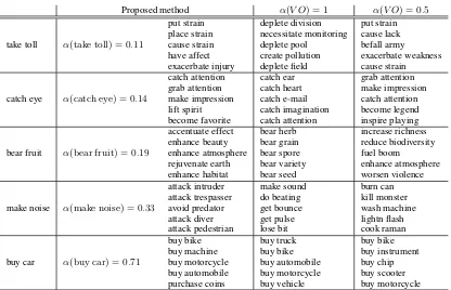
Table 5: Examples of the closest neighbors in the learned embedding space. All of the results were obtained by using the Wikipedia data, and the values ofα(V O)are the same as those in Table 2.

Method GS’11a GS’11b

Proposed method (Wikipedia) 0.598 0.461 Proposed method (BNC) 0.595 0.463 Proposed method (BNC-Wikipedia) 0.623 0.483 Proposed method (Ensemble A) 0.661 0.511 Proposed method (Ensemble B) 0.680 0.524

α(V O) = 0.5(Wikipedia) 0.491 0.386

α(V O) = 0.5(BNC) 0.599 0.462

α(V O) = 0.5(BNC-Wikipedia) 0.610 0.477

α(V O) = 0.5(Ensemble A) 0.612 0.474

α(V O) = 0.5(Ensemble B) 0.638 0.495

α(V O) = 1(Wikipedia) 0.576 n/a

α(V O) = 1(BNC) 0.574 n/a Milajevs et al. (2014) 0.456 n/a Polajnar et al. (2014) n/a 0.370 Hashimoto et al. (2014) 0.420 0.340 Polajnar et al. (2015) n/a 0.330 Grefenstette and Sadrzadeh (2011) n/a 0.210

Human agreement 0.750 0.620

Table 4: Transitive verb disambiguation task. The results forα(V O) = 1are reported in Hashimoto and Tsuruoka (2015).

with α(V O) = 1. We see that our method im-proves the baseline scores by adaptively combin-ing compositional and non-compositional embed-dings. Along with the results in Table 1, these re-sults show that our method allows us to improve the composition function by jointly learning non-compositional embeddings and the scoring

func-tion for composifunc-tionality detecfunc-tion.

6.2.2 Analysis of the Learned Embeddings We inspected the effects of adaptively weighting the compositional and non-compositional embed-dings. Table 5 shows the five closest neighbor phrases in terms of the cosine similarity for the three idiomatic phrases “take toll”, “catch eye”, and “bear fruit” as well as the two non-idiomatic phrases “make noise” and “buy car”. The exam-ples trained with the Wikipedia data are shown for our method and the two baselines, i.e.,α(V O) = 1 andα(V O) = 0.5. As shown in Table 2, the compositionality levels of the first three phrases are low and their non-compositional embeddings are dominantly used to represent their meaning.

adaptively using the non-compositional embed-dings.

The results ofα(V O) = 0.5are similar to those with our proposed method, but we can see some differences. For example, the phrase list for “make noise” of our proposed method captures offensive meanings, whereas that ofα(V O) = 0.5is some-what ambiguous. As another example, the phrase lists for “buy car” show that our method better cap-tures the semantic similarity between the objects thanα(V O) = 0.5. This is achieved by adaptively assigning a relatively large compositionality score (0.71) to the phrase to use the information about the object “car”.

We should note that “make noise” is highly compositional but our method outputs α(make noise) = 0.33, and the phrase list of α(V O) = 1 is the most appropriate in this case. Improving the compositionality detection function should thus further improve the learned embeddings.

7 Related Work

Learning embeddings of words and phrases has been widely studied, and the phrase embeddings have proven effective in many language process-ing tasks, such as machine translation (Cho et al., 2014; Sutskever et al., 2014), sentiment analysis and semantic textual similarity (Tai et al., 2015). Most of the phrase embeddings are constructed by word-level information via various kinds of composition functions like long short-term mem-ory (Hochreiter and Schmidhuber, 1997) recur-rent neural networks. Such composition functions should be powerful enough to efficiently encode information about all the words into the phrase embeddings. By simultaneously considering the compositionality of the phrases, our method would be helpful in saving the composition models from having to be powerful enough to perfectly encode the non-compositional phrases. As a first step to-wards this purpose, in this paper we have shown the effectiveness of our method on the task of learning verb phrase embeddings.

Many studies have focused on detecting the compositionality of a variety of phrases (Lin, 1999), including the ones on verb phrases (Diab and Bhutada, 2009; McCarthy et al., 2003) and compound nouns (Farahmand et al., 2015; Reddy et al., 2011). Compared to statistical feature-based methods (McCarthy et al., 2007; Venkatapathy

and Joshi, 2005), recent methods use word and phrase embeddings (Kiela and Clark, 2013; Yaz-dani et al., 2015). The embedding-based meth-ods assume that word embeddings are given in advance and as a post-processing step, learn or simply employ composition functions to com-pute phrase embeddings. In other words, there is no distinction between compositional and non-compositional phrases. Yazdani et al. (2015) fur-ther proposed to incorporate latent annotations (binary labels) for the compositionality of the phrases. However, binary judgments cannot con-sider numerical scores of the compositionality. By contrast, our method adaptively weights the com-positional and non-comcom-positional embeddings us-ing the compositionality scorus-ing function.

8 Conclusion and Future Work

We have presented a method for adaptively learn-ing compositional and non-compositional phrase embeddings by jointly detecting compositionality levels of phrases. Our method achieves the state of the art on a compositionality detection task of verb-object pairs, and also improves upon the pre-vious state-of-the-art method on a transitive verb disambiguation task. In future work, we will ap-ply our method to other kinds of phrases and tasks.

Acknowledgments

We thank the anonymous reviewers for their help-ful comments and suggestions. This work was supported by CREST, JST.

References

Mohit Bansal, Kevin Gimpel, and Karen Livescu. 2014. Tailoring Continuous Word Representations for Dependency Parsing. InProceedings of the 52nd Annual Meeting of the Association for Computa-tional Linguistics (Volume 2: Short Papers), pages 809–815.

Kyunghyun Cho, Bart van Merrienboer, Caglar Gul-cehre, Dzmitry Bahdanau, Fethi Bougares, Hol-ger Schwenk, and Yoshua Bengio. 2014. Learn-ing Phrase Representations usLearn-ing RNN Encoder– Decoder for Statistical Machine Translation. In Pro-ceedings of the 2014 Conference on Empirical Meth-ods in Natural Language Processing (EMNLP), pages 1724–1734.

Mona Diab and Pravin Bhutada. 2009. Verb Noun Construction MWE Token Classification. In Pro-ceedings of the Workshop on Multiword Expres-sions: Identification, Interpretation, Disambigua-tion and ApplicaDisambigua-tions, pages 17–22.

John Duchi, Elad Hazan, and Yoram Singer. 2011. Adaptive Subgradient Methods for Online Learning and Stochastic Optimization. Journal of Machine Learning Research, 12:2121–2159.

Meghdad Farahmand, Aaron Smith, and Joakim Nivre. 2015. A Multiword Expression Data Set: Annotat-ing Non-Compositionality and Conventionalization for English Noun Compounds. In Proceedings of the 11th Workshop on Multiword Expressions, pages 29–33.

Edward Grefenstette and Mehrnoosh Sadrzadeh. 2011. Experimental Support for a Categorical Composi-tional DistribuComposi-tional Model of Meaning. In Pro-ceedings of the 2011 Conference on Empirical Meth-ods in Natural Language Processing, pages 1394– 1404.

Kazuma Hashimoto and Yoshimasa Tsuruoka. 2015. Learning Embeddings for Transitive Verb Disam-biguation by Implicit Tensor Factorization. In Pro-ceedings of the 3rd Workshop on Continuous Vector Space Models and their Compositionality, pages 1– 11.

Kazuma Hashimoto, Pontus Stenetorp, Makoto Miwa, and Yoshimasa Tsuruoka. 2014. Jointly Learning Word Representations and Composition Functions Using Predicate-Argument Structures. In Proceed-ings of the 2014 Conference on Empirical Methods in Natural Language Processing (EMNLP), pages 1544–1555.

Sepp Hochreiter and J¨urgen Schmidhuber. 1997. Long Short-Term Memory. Neural Computation, 9(8):1735–1780.

Dimitri Kartsaklis, Mehrnoosh Sadrzadeh, and Stephen Pulman. 2012. A Unified Sentence Space for Categorical Distributional-Compositional Seman-tics: Theory and Experiments. In Proceedings of the 24th International Conference on Computational Linguistics, pages 549–558.

Dimitri Kartsaklis, Nal Kalchbrenner, and Mehrnoosh Sadrzadeh. 2014. Resolving Lexical Ambiguity in Tensor Regression Models of Meaning. In Proceed-ings of the 52nd Annual Meeting of the Association for Computational Linguistics (Volume 2: Short Pa-pers), pages 212–217.

Douwe Kiela and Stephen Clark. 2013. Detecting Compositionality of Multi-Word Expressions using Nearest Neighbours in Vector Space Models. In

Proceedings of the 2013 Conference on Empirical Methods in Natural Language Processing, pages 1427–1432.

Geoffrey Leech. 1992. 100 Million Words of English: the British National Corpus. Language Research, 28(1):1–13.

Omer Levy and Yoav Goldberg. 2014. Dependency-Based Word Embeddings. In Proceedings of the 52nd Annual Meeting of the Association for Compu-tational Linguistics (Volume 2: Short Papers), pages 302–308.

Dekang Lin. 1999. Automatic Identification of Non-compositional Phrases. InProceedings of the 37th Annual Meeting of the Association for Computa-tional Linguistics, pages 317–324.

Diana McCarthy, Bill Keller, and John Carroll. 2003. Detecting a Continuum of Compositionality in Phrasal Verbs. In Proceedings of the ACL 2003 Workshop on Multiword Expressions: Analysis, Ac-quisition and Treatment, pages 73–80.

Diana McCarthy, Sriram Venkatapathy, and Aravind Joshi. 2007. Detecting Compositionality of Verb-Object Combinations using Selectional Preferences. In Proceedings of the 2007 Joint Conference on Empirical Methods in Natural Language Process-ing and Computational Natural Language LearnProcess-ing, pages 369–379.

Tomas Mikolov, Ilya Sutskever, Kai Chen, Greg S Cor-rado, and Jeff Dean. 2013. Distributed Representa-tions of Words and Phrases and their Composition-ality. InAdvances in Neural Information Processing Systems 26, pages 3111–3119.

Dmitrijs Milajevs, Dimitri Kartsaklis, Mehrnoosh Sadrzadeh, and Matthew Purver. 2014. Evaluating Neural Word Representations in Tensor-Based Com-positional Settings. InProceedings of the 2014 Con-ference on Empirical Methods in Natural Language Processing, pages 708–719.

Jeff Mitchell and Mirella Lapata. 2008. Vector-based Models of Semantic Composition. InProceedings of 46th Annual Meeting of the Association for Com-putational Linguistics: Human Language Technolo-gies, pages 236–244.

Yusuke Miyao and Jun’ichi Tsujii. 2008. Feature For-est Models for Probabilistic HPSG Parsing. Compu-tational Linguistics, 34(1):35–80, March.

Masayasu Muraoka, Sonse Shimaoka, Kazeto Ya-mamoto, Yotaro Watanabe, Naoaki Okazaki, and Kentaro Inui. 2014. Finding The Best Model Among Representative Compositional Models. In

Proceedings of the 28th Pacific Asia Conference on Language, Information, and Computation, pages 65–74.

Mark Newton. 2006. Basic English Syntax with Exer-cises. B¨olcs´esz Konzorcium.

Jeffrey Pennington, Richard Socher, and Christopher Manning. 2014. Glove: Global Vectors for Word Representation. In Proceedings of the 2014 Con-ference on Empirical Methods in Natural Language Processing (EMNLP), pages 1532–1543.

Nghia The Pham, Germ´an Kruszewski, Angeliki Lazaridou, and Marco Baroni. 2015. Jointly opti-mizing word representations for lexical and senten-tial tasks with the C-PHRASE model. In Proceed-ings of the 53rd Annual Meeting of the Association for Computational Linguistics and the 7th Interna-tional Joint Conference on Natural Language Pro-cessing (Volume 1: Long Papers), pages 971–981.

Tamara Polajnar, Laura Rimell, and Stephen Clark. 2014. Using Sentence Plausibility to Learn the Semantics of Transitive Verbs. In Proceedings of Workshop on Learning Semantics at the 2014 Con-ference on Neural Information Processing Systems.

Tamara Polajnar, Laura Rimell, and Stephen Clark. 2015. An Exploration of Discourse-Based Sentence Spaces for Compositional Distributional Semantics. In Proceedings of the First Workshop on Linking Computational Models of Lexical, Sentential and Discourse-level Semantics, pages 1–11.

Siva Reddy, Diana McCarthy, and Suresh Manandhar. 2011. An Empirical Study on Compositionality in Compound Nouns. InProceedings of 5th Interna-tional Joint Conference on Natural Language Pro-cessing, pages 210–218.

Richard Socher, Brody Huval, Christopher D. Man-ning, and Andrew Y. Ng. 2012. Semantic Compo-sitionality through Recursive Matrix-Vector Spaces. In Proceedings of the 2012 Joint Conference on Empirical Methods in Natural Language Process-ing and Computational Natural Language LearnProcess-ing, pages 1201–1211.

Ilya Sutskever, Oriol Vinyals, and Quoc V Le. 2014. Sequence to Sequence Learning with Neural Net-works. InAdvances in Neural Information Process-ing Systems 27, pages 3104–3112.

Kai Sheng Tai, Richard Socher, and Christopher D. Manning. 2015. Improved Semantic Representa-tions From Tree-Structured Long Short-Term Mem-ory Networks. InProceedings of the 53rd Annual Meeting of the Association for Computational Lin-guistics and the 7th International Joint Conference on Natural Language Processing (Volume 1: Long Papers), pages 1556–1566.

Tim Van de Cruys. 2014. A Neural Network Approach to Selectional Preference Acquisition. In Proceed-ings of the 2014 Conference on Empirical Methods in Natural Language Processing (EMNLP), pages 26–35.

Sriram Venkatapathy and Aravind Joshi. 2005. Mea-suring the Relative Compositionality of Verb-Noun

(V-N) Collocations by Integrating Features. In Pro-ceedings of Human Language Technology Confer-ence and ConferConfer-ence on Empirical Methods in Nat-ural Language Processing, pages 899–906.