Munich Personal RePEc Archive
Incremental Risk Charge Methodology
Xiao, Tim
BMO
8 May 2019
Online at
https://mpra.ub.uni-muenchen.de/94581/
Incremental Risk Charge Methodology
Tim Xiao
1ABSTRACT
The incremental risk charge (IRC) is a new regulatory requirement from the Basel
Committee in response to the recent financial crisis. Notably few models for IRC have been
developed in the literature. This paper proposes a methodology consisting of two Monte Carlo
simulations. The first Monte Carlo simulation simulates default, migration, and concentration in
an integrated way. Combining with full re-valuation, the loss distribution at the first liquidity
horizon for a subportfolio can be generated. The second Monte Carlo simulation is the random
draws based on the constant level of risk assumption. It convolutes the copies of the single loss
distribution to produce one year loss distribution. The aggregation of different subportfolios with
different liquidity horizons is addressed. Moreover, the methodology for equity is also included,
even though it is optional in IRC.
Keywords: Incremental risk charge (IRC), constant level of risk, liquidity horizon, constant loss
distribution, Merton-type model, concentration.
1
Introduction
1Address correspondence to Tim Xiao, Risk Quant, Capital Markets, CIBC, 161 Bay Street, Toronto, ON
The Basel Committee on Banking Supervision (see Basel [2009 a]) released the new
guidelines for Incremental Risk Charge (IRC) that are part of the new rules developed in response
to the financial crisis and is a key part of a series of regulatory enhancements being rolled out by
regulators.
IRC supplements existing Value-at-Risk (VaR) and captures the loss due to default and
migration events at a 99.9% confidence level over a one-year capital horizon. The liquidity of
position is explicitly modeled in IRC through liquidity horizon and constant level of risk.
The constant level of risk assumption in IRC reflects the view that securities and
derivatives held in the trading book are generally more liquid than those in the banking book and
may be rebalanced more frequently than once a year. IRC should assume a constant level of risk
over a one-year capital horizon which may contain shorter liquidity horizons. This constant level
of risk assumption implies that a bank would rebalance, or rollover, its positions over the
one-year capital horizon in a manner that maintains the initial risk level, asindicated by the profile of
exposure by credit rating and concentration.
The current market risk capital rule is:
Total market risk capital = general market risk capital
+ basic specific risk capital (1)
+ specific risk surcharge
where
General market risk capital = 3 x General _VaR9910%day
Basic specific risk capital = 3 x
Specific
_
VaR
9910%daySpecific risk surcharge = (m – 3) x
Specific
_
VaR
9910%daywhere m is the specific risk capital multiplier under regulators’ guidance
Total market risk capital = general market risk capital
+ basic specific risk capital (2)
+ incremental risk charge
where Incremental risk charge =
IRC
_
VaR
991.year9%In this paper, we present a methodology for calculating IRC. First, a Merton-type model
is introduced for simulating default and migration. The model is modified to incorporate
concentration. The calibration is also elaborated. Second, a simple approach to determine market
data, including equity, in response to default and credit migration is presented. Next, a
methodology toward constant level of risk is described. The details of applying the constant level
of risk assumption and aggregating different subportfolios are addressed. Finally, the empirical
and numerical results are presented.
2
Simulation of Default and Credit Migration
The IRC encompasses all positions subject to a capital charge for specific interest rate
risk according to the internal models with exception of securitization and nth-to-default credit
derivatives. Equity is optional. For IRC-covered positions, the IRC captures default risk and
credit migration risk only.
2.1 Simulation Model
Most of the portfolio models of credit risk used in the banking industry is based on the
conditional independence framework. In these models, defaults and credit migration of individual
borrowers depend on a set of common systematic risk factors describing the state of the economy.
Merton-type models have become very popular. The Merton-type model (or standardized Merton
model) is
i i i
i
z
1
2
(3)i
, The independent standard normally random variables
The systematic riski
The idiosyncratic risk for issuer/obligor ii
The weighted correlation reflecting the impact of systematic risk factoron issuer/obligor i.
i
z The normalized asset return or creditworthiness indicator for
issuer/obligor i
This model becomes the most popular one in default and migration risk modeling and
yields the core of the Basel II capital rule (see Heitfield [2003]).
Similar to the original Merton model, this model is also assuming that the default and
migration only happens at the end, which achieves significant simplification.
2.2 Simulation model for multiple-liquidity-horizon subportfolios
Liquidity horizons are determined for each position to reflect actual practice and
experience during periods of both systematic and idiosyncratic stresses. The total portfolio shall
be divided into the subportfolios based on different liquidity horizons. Let’s assume that there are
two subportfolios with different liquidity horizons: 3 month and 6 month. To model different
liquidity periods, one can use the above model (3) but calibrate different
i’s, such as,
3m_iand
6m_i, for different periods.Alternatively, one can also use a multiple-period model as:
i m i m
i m
z3
3 1
2
3 _ For 3 month (4)i m i m
m i m
z 6 _
2 2
3 6
6 1
1
For 6 month (5)
where
i is unique for different periods under issuer i and
is an exponentially declining2.3 Calibration of
iThe most popular approaches to calibrate the asset correlation are Maximum Likelihood
Estimation or regression based on time series default data. Alternatively, in the new Basel Capital
Accord, a formula for derivation of risk weighted asset correlation for corporate, sovereign, and
bank exposures is given as (see Tasche [2004] and Basel [2003]):
) 1 ( 24 . 0 12
.
0 i i
i
(6)Where 50
50
1 1
e e PDi
i
2.4 Concentration
The phenomenon we need to model is that concentration will result a higher IRC number,
comparing to non-concentration case. Furthermore, the more concentration a portfolio has, the
higher IRC result it generates. To achieve this, we model the effect of issuer and market
concentration as well as clustering of default and migration by introducing another parameter, the
concentration parameter.
There are two correlations we need to consider: correlation between credit migration and
default events of obligors and correlation between credit migration/default events and systematic
market risk factors. The study (see Kim [2009]) shows that the correlation between credit
migration/default events and systematic market risk factors is very small and negligible.
However, correlation between credit migration and default events of obligors is significant and
cannot be ignored. Therefore, the concentration parameter is solely dependent on correlation
between credit migration and default.
Our methodology is based on a simple mechanism for coupling issuer/market
concentrations to migrations and defaults. In the simulation framework (3) or (4) and (5), the
probability of a migration or default increases with the asset volatility. Since the effect of
within that sector, we model increased concentration as an increase in the volatility of the
systematic risk driver. All positions sensitive to that risk driver will have an increased probability
of migration/default events occurring. The modified simulation model is
i i t i i i
z
(1 |
|)
1
2
(7a)Where
i is the weighted concentration factor depending on correlation between issuer defaultand migration events and
k k t k t t t
x
x
x
2 2 11
(7b)where if one uses (3),
= 0 and
t xt
. Otherwise,
is time declining weight andk t
t x
x,, are independent standard normally random variables representing systematic risks in different time periods.
2.5 Calibration of
iThe calibration is based on credit migration matrix. It can be derived using either analytic
closed-form or Monte-Carlo simulation. In theory, one can use Pearson’s product moment or
Kendall’s
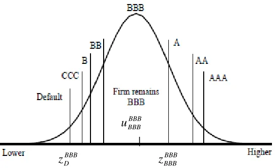
.2.6 Determination of default and credit migration
The simulated asset return zi, combined with migration/default thresholds, is used to
ascertain when default or migration is deemed to occur. The calculation of the thresholds of credit
migration and default is based on credit migration probability (see JP Morgan [1997]). Using a
BBB issuer as an example and given migration matrix, we can calculate the thresholds as:
BBB AA BBB A BBB BBB BBB BB BBB B BBB CCC BBB
D
z
z
z
z
z
z
Figure 1 Credit migration rating thresholds (for BBB)
If the normalized asset of the issuer is smaller than BBB D
z , it defaults. If the normalized
asset is between BBB D
z and BBB CCC
z , it migrates to CCC, and so on. We use an effective middle value
to represent each band:
21((
(
)
0
)
1
BBBD BBB
D
z
u
21((
(
)
(
))
1 BBB
D BBB
CCC BBB
CCC
z
z
u
21((
(
)
(
))
1 BBB
B BBB
CCC BBB
B
z
z
u
21((
(
)
(
))
1 BBB
BB BBB
B BBB
BB
z
z
u
(8)
21((
(
)
(
))
1 BBB
BBB BBB
BB BBB
BBB
z
z
u
21((
(
)
(
))
1 BBB
A BBB
BBB BBB
A
z
z
u
21((
(
)
(
))
1 BBB
AA BBB
A BBB
AA
z
z
u
21((
(
)
1
)
1
BBBAA BBB
AAA
z
u
2.7 Calibration of transition matrix, default probability (PD), and loss given
default (LGD)
BBB D
z zBBBBBB
BBB BBB
The straight forward cohort approach is used to estimate transition matrices based on
obligors’ rating history, which has become the industry standard. The PD estimate is based on
EDF data that is used for calculation of PD benchmarked against internal default history. Internal
data is used for LGD parameter benchmarked against relevant external proxy data.
3
Credit Spreads and Equity Prices
After simulating default and migration of all issuers/obligors, we need to price every
instrument in order to generate loss distributions. The question is whether we should simulate
market data or not?
The earlier version of Basel IRC paper (see Basel [2008]) requires financial institutes to
capture four risks: default, credit migration, significant credit spread changes, and significant
equity price changes. However, the new guideline (see Basel [2009 a]) limits the risks to default
and credit migration only. In addition, a separate Basel paper (see Basel [2009 b]) further states
that IRC contains only incremental default and migration risks, and all price risks belong to the
comprehensive risk. These messages give us a clear indication that only default and credit
migration are risk factors in IRC and all market prices/data are not. Therefore, we recommend
simulating default and migration only but not simulating any market prices/data.
We assume all market prices/data are deterministic (flat) and use forward prices/data for
valuation. The fat tail behavior and market correlations are embedded in the market. Keeping
these parameters constant ensures we measure only P&L variation due to credit rating changes
(migration or default) per IRC requirements. The selection of credit spreads or equity prices,
however, should reflect the credit quality changes.
All issuers/obligors shall be divided into credit groups based on geographies and sectors.
Assume that the credit spreads for different ratings under each group are available. Then we can
select associated credit spreads to price a bond or a CDS according to the creditworthiness
simulation of the issuer/obligor.
3.2 Equity prices
In risk neutral world, the forward equity price at future time T is
rT
T
E
e
E
0 (9)Where r is the risk free interest rate and E0 is the today’s spot equity price
If the issuer defaults at T, the equity price should be 0. If the issuer is upgraded or
downgraded, the equity price should be larger or smaller than the risk neutral forward price
rT
T
E
e
E
0 . This is the phenomenon we are going to model: downgraded if e E upgraded if e E default if change credit no if e E E rT o rT rT T 0 0 0 (10)
The underlying dynamic of Merton model is
t t A t
t rAdt AdW
dA
(11)Where At is the corporate asset value; r is the risk-free interest rate;
A is the asset volatilityand Wt is the Wiener process.
Applying Ito’s lemma, we have
rT T Ty
AAT 21
A2
A0exp (12)
where y denote the standard normal variable
The Merton model states that the equity of a company is a European call option on the
asset of the company with maturity T and a strike price equal to the face value of the debt that
The payoff of Merton model is
,
0
max
A
D
E
T
T
(13)where D denotes the debt of the company.
The mathematical expression of Merton model is
)
(
)
(
1 20
0
A
N
d
e
DN
d
E
rT (14)where
d
A
D
rT
AT
A
2
1
)
/
ln(
0 2 , 1
We still use the BBB issuer as an example. Based on (8), (12), and (13), the equity price
at T, if default occurs, is
0
exp
21 20
D
u
T
T
rT
A
D
A
E
TBBB D TD
A
A DBBB (15)The equity price at T without credit quality changes is
BBB
rTBBB A A BBB T BBB BBB
T
A
D
A
rT
T
T
u
D
E
e
E
21 2 00
exp
(16)We solve equations (14), (15), and (16) to get A0,
A, and D. Then, with the known A0,A
, and D, we can obtain any equity price at T under any credit rating according to (8) and (13).For instance, when the rating changes from BBB to A, the equity price at T is
rT
T
T
u
D
A
D
A
E
TBBBA
TA
21
A2
A BBBA
0exp
)
0
,
max(
(17)4
Constant Level of Risk
The constant level of risk reflects recognition by regulators that securities/derivatives
held in the trading book are generally much more liquid than those in the banking book, where a
buy-and-hold assumption over one year may be reasonable. It implies that IRC should be
modeled under the assumption that banks rebalance their portfolio several times over the capital
horizon in order to maintain a constant risk profile as market conditions evolve. Of course, we do
behavior: clearly portfolios are altered on a daily basis, not simply held constant for some period
then instantaneously rebalanced. Rather, we regard the rollover interpretation as being a
reasonable approximation to the way banks manage their trading portfolios over a certain
horizon. In general, one should model constant level of risk instead of constant portfolio over one
year capital horizon.
There are several ways to interpret constant level of risk: constant loss distribution or
constant risk metrics (e.g. VaR). We believe the constant loss distribution assumption is the most
rigorous. Under this assumption, the same metrics (e.g. VaR, moments, etc.) can be achieved for
each liquidity horizon.
The liquidity horizon for a position or set of positions has a floor of three months. Let us
use three months as an example. We interpret constant level of risk to mean that the bank holds
its portfolio constant for the liquidity horizon, then rebalances by selling any default,
downgraded, or upgraded positions and replaces them so that the portfolio is returned to the level
of risk it had at the beginning. The process is repeated 4 times over the capital horizon resulting 4
independent and identical loss distributions. The one year constant level of risk loss distribution is
the convolution of 4 copies of the three month loss distribution. In Monte Carlo context, this
can be modeled by drawing 4 times from the single period loss distribution measured over
the liquidity horizon. The total PnL is the summary of these 4 random draws.
An intuitive explanation is shown in Figure 2. A generic path with appears in red; P&L
contributions from each liquidity horizon appear in blue. In this schematic, the position
experiences downgrade, upgrade or default, resulting in a loss or profit. This position is then
removed and replaced at the end of each liquidity horizon by rebalancing. The final P&L for the
path will be the summary of all losses and profits.
Portfolio
Figure 2 Constant level of risk
In addition, one needs to consider the reinvestment of all cash flows realized during the
liquidity horizon and rollover of expired deals.
5
Aggregation and Time Horizon Correlation
First we need to divide the portfolio into the subportfolios based on liquidity horizons. If
there is only one single-liquidity-horizon subportfolio, the rebalance at the end of each liquidity
horizon washes out the time horizon correlation. However, if there are multiple subportfolios, the
time horizon correlations need to be addressed.
To elaborate the details, we assume there are two subportfolios with liquidity horizons: 3
months and 6 months. Based on the default and migration simulation and full re-valuation, we
can generate loss distributions at first liquidity horizons for 3-month and 6-month subportfolios as
m
PL3 , and PL6m.
There are two approaches to achieve the correlative aggregation: copula approach or
correlation matrix approach.
We conduct the second Monte Carlo simulation by generate 4 standard normal random
draws for scenario j:
x
1j,
x
2j,.
x
3j,
x
4j. These random draws represent a Monte-Carlo path.5.1.1 Three-month Subportfolio
The P&L distribution of three-month subportfolio is PL3m. The four draws of loss
distribution are 3
(
1)
,
3
(
2)
,
3
(
3)
,
3
(
4j)
m j m j m j
m
x
PL
x
PL
x
PL
x
PL
, where
is theaccumulative normal. The total P&L of the three-month subportfolio for scenario j is
4 1 3 3 _ ( ) i j i m j mtotal PL x
PL (18)
5.1.2 Six-month Subportfolio
The P&L distribution of the six-month subportfolio is PL6m. We can calculate
correlation
(PL3m,PL6m) between PL3m and PL6m using Pearson product-moment. The twocorrelated random draws are m m j
j m m j
m PL PL x PL PL x
x6 _1
( 3 , 6 ) 1 1
( 3 , 6 )2 2 andj m m j m m j
m PL PL x PL PL x
x6 _2
( 3 , 6 ) 3 1
( 3 , 6 )2 4. The two draws of loss distribution are
(
6 _1)
,
6
(
6 _2)
6 j m m j m
m
x
PL
x
PL
. The total P&L of the six-month subportfolio for scenario j is
2 1 _ 6 6 6 _ ( ) i j i m m j mtotal PL x
PL (19)
Summing up (18) and (19), we can get the total P&L for scenario j as
j m total j m total j
total
PL
PL
PL
_6
_3 (20)5.2 Correlation matrix approach
Based on the four 3-month independent identical loss distributions:
m m m
m PL PL PL
PL3 , 3 , 3 , 3 , and two 6-month independent identical loss distributions:
m
m PL
Cholesky decomposition to the correlation matrix
, we have
LL
T, where L is a lowertriangular matrix.
We conduct the second Monte Carlo simulation by generating 4 independent standard
normal random draws:
x
1j,
x
2j,.
x
3j,
x
4j for the four 3-month periods in a year and 2 independentstandard normal random draws j
x5,
j
x6 for the two 6-month periods to construct a path/scenario j.
The random draw vector is
X
x
1jx
2jx
3jx
4jx
5jx
6j
. We can obtain correlativerandom draw vector
j j j j j j
x
x
x
x
x
x
X
~
~
1~
2~
3~
4~
5~
6 by X~T LXT (21) The total P&L for scenario j is
6 5 6 4 1 3 6 _ 3 _ (~ ) (~ ) i j i m i j i m j m total j m total jtotal PL PL PL x PL x
PL (22)
The final IRC will be 99.9% VaR based on distribution j total
PL . In general, the
correlation matrix approach is more generic and can be easily extended to any number of
subportfolios.
6
Numerical and Empirical Results
The above methodology has been implemented. The empirical study shows the results on
P&L distributions, numerical stability & convergence, concentration effect, and capital impact.
pdf: 3 month loss distribution
0 0.001 0.002 0.003 0.004 0.005 0.006 0.007 0.008 0.009
-1000 -800 -600 -400 -200 0 200 400 600 800 1000
loss / 10,000
[image:16.612.169.444.75.250.2]Figure 3 Histogram of loss distribution at 3 month
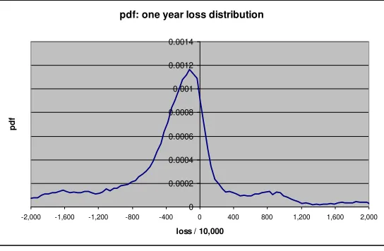
pdf: one year loss distribution
0 0.0002 0.0004 0.0006 0.0008 0.001 0.0012 0.0014
-2,000 -1,600 -1,200 -800 -400 0 400 800 1,200 1,600 2,000
loss / 10,000
[image:16.612.170.442.316.494.2]Figure 4 Histogram of loss distribution at 1 year
6.1 Convergence study
People normally believe that 50,000 simulations provide sufficient stability to measure
the 99.9th percentile loss required for the regulatory IRC measure. However, our study shows that
50,000 paths are not convergent. Actually 100,000 simulations are needed to archive a better
numerical stability and convergence. The results are shown in Table 1
Scenarios IRC Diff from previous Diff from average
8,000.00 102.31 -1.51%
10,000.00 103.56 1.23% -0.30%
20,000.00 100.44 -3.01% -3.30%
40,000.00 100.71 0.27% -3.04%
60,000.00 110.01 9.23% 5.91%
80,000.00 105.22 -4.35% 1.30%
100,000.00 104.90 -0.31% 0.99%
120,000.00 103.66 -1.18% -0.20%
140,000.00 103.96 0.28% 0.08%
160,000.00 103.61 -0.33% -0.25%
180,000.00 105.23 1.56% 1.31%
200,000.00 103.14 -1.99% -0.71%
Average 103.87
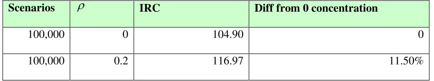
6.2 Concentration study
The purpose of this section is to demonstrate that the model (7) can reflect issuer and
market concentrations. To simplify our tests, we assign all issuers with the same concentration
factor
. It is shown that the IRC increases according to the increasing of
, up to 30% in table [image:17.612.82.504.639.718.2]2.
Table 2 Concentration study
Scenarios
IRC Diff from 0 concentration100,000 0 104.90 0
100,000 0.4 122.37 16.66%
100,000 0.6 128.49 22.48%
100,000 0.8 132.83 26.63%
100,000 1 137.23 30.82%
6.3 Capital impact
The capital impact can be measured as the ratio between IRC and specific risk surcharge.
The results significantly depend on the composition of a portfolio and the specific risk multiplier
of a financial institution set by the regulator. The ratio of our testing portfolio is 5.8.
References
Basel Committee on Banking Supervision, 31 July 2003, “The new Basel capital accord.”
Basel Committee on Banking Supervision, July 2008, “Guidelines for Computing Capital for
Incremental Default Risk in the Trading Book.”
Basel Committee on Banking Supervision, July 2009 (a), “Guidelines for Computing Capital for
Incremental Risk in the Trading Book.”
Basel Committee on Banking Supervision, July, 2009 (b), “Revisions to the Basel II market risk
framework.”
Basel Committee on Banking Supervision, October 2009 ©, “Analysis of the trading book
Gary Dunn, April 2008, “A multiple period Gaussian Jump to Default Risk Model.”
FinPricing, Risk Management Solution, https://finpricing.com/paperList.html
Erik Heitfield, 2003, “Dealing with double default under Basel II,” Board of Governors of the
Federal Reserve System.
Jongwoo Kim, Feb 2009, “Hypothesis Test of Default Correlation and Application to Specific
Risk,” RiskMetrics Group.
J.P.Morgan, April, 1997, “CreditMetrics – Technical Document.”
Dirk Tasche, Feb 17, 2004, “The single risk factor approach to capital charges in case of
correlated loss given default rates.”
Tim Xiao, February 2009, “Incremental Risk Charge Methodology,” CIBC Internal.