Squaring the energy efficiency circle: evaluating industry energy efficiency policy in a hybrid model setting

Munich Personal RePEc Archive

Squaring the energy efficiency circle:

evaluating industry energy efficiency

policy in a hybrid model setting

Andersen, Kristoffer Steen and Dockweiler, Steffen and

Klinge Jacobsen, Henrik

Technical University of Denmark, DTU Management, Energy

Economics and Regulation, The Danish Energy Agency

September 2019

Online at

https://mpra.ub.uni-muenchen.de/96546/

WORKING PAPER September 2019

Squaring the energy efficiency circle: evaluating industry energy

efficiency policy in a hybrid model setting

Kristoffer S. Andersena,b,_∗

, Steffen Dockweilerb

, Henrik Klinge Jacobsena

a

Technical University of Denmark, DTU Management, Produktionstorvet, Building 424, 2800 Kongens Lyngby, Denmark

b

The Danish Energy Agency, Carsten Niebuhrs Gade 43, 1577 Copenhagen, Denmark

Abstract

Improving energy efficiency within the industry will play a central role in mitigating green-house gas emissions by reducing the use of fossil fuels. Nevertheless, the ex-ante evaluation of energy-efficiency policies largely remains an unresolved challenge. Understood within a theoretical economic framework, the root of the challenge is the simultaneity and interac-tion between three primary effects: an activity, a price, and a technical effect. This paper demonstrates how the IntERACT model, a Danish hybrid model, captures each effect and their interactions endogenously. The paper finds that a specific energy efficiency policy leads to an additional reduction in industrial energy use of around 5% in the year 2030, of which a policy-induced reduction in the energy efficiency gap accounts for half. The results reflect a total rebound effect of 12.5% and an implied elasticity of energy service demand of around 15% across industrial sectors.

Keywords: Energy systems analysis, sectoral energy efficiency modelling, energy efficiency policies, energy savings

1. Introduction

The International Energy Agency’s Energy Technology Perspectives proclaims that en-ergy efficiency will need to deliver 55 pct. of cumulative global industrial CO_2–emission

reductions between now and 2060 to ensure that the global temperature increase remains below 2 degrees above pre-industrial levels (IEA, 2017). Despite such claims, evaluating the future role of energy efficiency is a considerable challenge. The extent of the challenge be-comes apparat in the body of literature discussing issues such as the additionality of energy

∗_{Corresponding author}

efficiency policies, the energy efficiency gap, and the rebound effects associated with energy efficiency policies.

For example, when assessing the additionality of an energy efficiency policy, determining the energy efficiency baseline becomes a critical challenge (Vine, 2008). Identifying and removing the energy efficiency gap, i.e., the existence of significant unexploited and cost-effective opportunities for energy efficiency investment (Koopmans and Te Velde, 2001), demands careful consideration when it comes to the types of barrier responsible for the gap and the type of policies that could reduce the gap. Finally, assessing the rebound effect of energy efficiency policies is of great importance when evaluating the effectiveness of such policies (Barker et al., 2007b; Sorrell, 2009).

Our research objective is to show how it is possible to address these issues systemat-ically when conducting ex-ante evaluations of energy efficiency policies within a modeling framework. The paper is structured as follows. Section 2 develops a microeconomic ana-lytical framework for understanding the industry’s energy service demand decision. Section 3 reviews the literature on ex-ante modeling of energy efficiency and assesses the extent to which the literature captures the different components of the energy service demand deci-sion. Section 4 describes the Danish IntERACT model, which is the comprehensive hybrid model used in this paper. Section 5 presents and discusses results related to both a baseline and an energy efficiency policy scenario, demonstrating how IntERACT solves the three key challenges of energy efficiency modeling. Section 6 concludes.

2. Analytical background

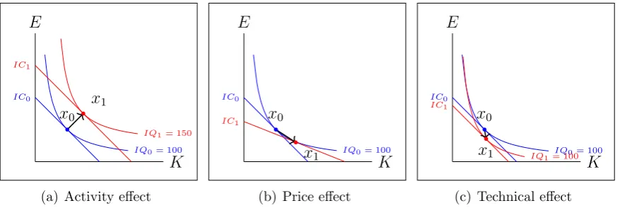
Energy is a derived demand, not required for its own sake, but for the energy ser-vices it provides to households and businesses (Hunt and Ryan, 2015). Following Filippini and Hunt (2015), we treat energy services as the combination of energy and other inputs (mainly capital, e.g., boiler technology and insulation) that produce the desired service (e.g., a comfortable room temperature). The economic theory of cost and production provides a framework for understanding firms’ energy service demand decisions (Berndt (1990); Hunt-ington (1994)). Figure 1a-c illustrates the application of this framework to the energy service demand decision within a sector, i.e., the situation in which a sector uses capital (K) and en-ergy (E) to derive an enen-ergy service. The enen-ergy service production technology and relative input prices are represented using isoquant curves (IQ) and isocost lines (IC), respectively. We note that energy services serve as a further input to an overall production function (not shown in Figure 1), which also includes labor, materials, and non-energy-service related capital.

Figure 1: Isoquant representation of the energy service demand decision

K E

IQ0= 100

IC0

IQ1= 150

IC1

x₀ x₁

(a) Activity effect

K E

IQ0= 100

IC0

IC1

x₀

x₁

(b) Price effect

K E

IQ0= 100

IC0

IQ1= 100

IC1

x₀

x₁

(c) Technical effect

We assume that energy services are produced in a cost-efficient manner, conditioned on the existing production technology (isoquant curve) and the perceived input costs (isocost line). In period t, point x0 illustrates the cost-minimizing input combination, where the

isocost line (IC0) is tangent to the isoquant (IQ=100). We do not rule out the existence

of inefficiencies in energy service production arising from, e.g., an energy efficiency gap or the distortionary effect of energy taxes. However, for now, we consider these inefficiencies as embedded in the isoquant curves and isocost lines.

The activity effect (Figure 1a) captures the isolated effect of an increase in the energy ser-vice demand at the sectoral level while keeping the relative price and production technology fixed. The activity effect may arise from overall economic growth or structural adjustments leading to a change in the activity of the particular sector. Under an assumption of constant returns to scale in energy service production, the activity effect will not impact the energy intensity or energy efficiency of energy service supply within the sector. However, the activ-ity effect may impact the economy-wide energy intensactiv-ity and energy efficiency if the sectoral composition of the economy changes as a result of, for example, a relative decrease in the activity of energy-intensive sectors.

The price effect (Figure 1b) captures energy service input substitution related to the change in the relative prices. Figure 1b illustrates the input substitution as the relative price of capital is reduced (the move from IC0 to IC1). By its nature, the price effect may impact

the energy intensity by shifting the relative shares of capital and energy in the production of energy services1_{. We note that the price effect, as discussed above, overlaps with what}

Greening et al. (2000) term the direct rebound, whereas the activity effect corresponds to the indirect rebound and the economy-wide rebound (ibid.).

Finally, the technical effect (Figure 1c) captures the deployment of new energy service production technology; for example, a highly efficient heat pump replacing an older inefficient oil boiler in period t+1. Figure 1c illustrates the technical effect as the change in production

1_{Understood within a somewhat broader general equilibrium context the price effect also captures the}

technology from IQ0 to the IQ1 isoquant. Both of these production technologies represent

the same output of energy service. As a result, energy service production becomes both more energy-efficient and more capital intensive (even in absolute terms) in period t+1. The technical effect can materialize as incremental efficiency improvement, e.g., a slightly more efficient boiler, but it can also reflect a more fundamental capital substitution, i.e., investment in insulation or process optimization reducing the overall need for fuel.

In practice, the activity, price, and technical effects are simultaneous, and they interact. For example, a price effect may incur second-order interaction effects in terms of activity effect (e.g., indirect and economy-wide rebound effects) or technical effects (e.g., as prices may change the trade-off associated with the investment in different energy service technolo-gies). Ignoring the second-order activity effect neglects part of the rebound effect. Leaving out the second-order technical effects risks overlooking issues such as the path dependency of investments in energy service conversion technologies. Overall, leaving out any of these interaction effects makes it challenging to construct a baseline as the baseline ideally needs to account for each effect as well as the interactions between them.

3. Literature review

The literature on the ex-ante evaluation of energy efficiency policies for industrial sectors is sparse. Concerning EU energy efficiency policies, Rosenow et al. (2016) observe that no peer-reviewed ex-ante evaluations are available. Instead, ex-ante evaluations of energy efficiency policies tend to focus on heating and appliances in households (see, e.g., Mundaca et al. (2010). Due to the scarcity of ex-ante evaluations of energy efficiency policies for industry, this review focuses more broadly on the ex-ante modeling of industrial energy efficiency. We approach the literature by discussing the extent to which existing studies capture the technical, price, and activity effects. By doing so, we highlight the fragmented nature of the field, which reflects the tendency of most studies to only focus on a subset of the three effects. Studies usually follow either a bottom-up approach, which focuses on the technical effect (largely ignoring the price and activity effect) or a top-down approach, which typically focuses on the demand side (in terms of price and activity effects), describing the technical effect endogenously. Although hybrid models that combine components of the top-down and bottom-up approaches exist, we have not been able to find examples of any that capture all three effects simultaneously, including second-order interaction effects. Table 1 presents a summary of our findings.

3.1. Capturing the technical effect

Table 1: Review of ex-ante energy efficiency studies on industrial sectors

Study Model type Technical effect Price effect Activity effect Interaction effects Bataille et al. (2006) Bottom-up Endogenous Partly endogenous Partly endogenous No McNeil et al. (2013) Bottom-up Exogenous Exogenous Exogenous No Loulou et al. (2016) Bottom-up Endogenous Partly endogenous Partly endogenous No Grepperud and Rasmussen (2004) Top-down Exogenous Endogenous Endogenous No Hanley et al. (2006) Top-down Exogenous Endogenous Endogenous No Allan et al. (2007) Top-down Exogenous Endogenous Endogenous No Barker et al. (2007b)1 _{Top-down Exogenous Exogenous Endogenous No} Barker et al. (2007a)1 _{Top-down Exogenous Exogenous Endogenous No} Barker et al. (2009)1 _{Top-down Exogenous Exogenous Endogenous No} Bataille and Melton (2017) Top-down Exogenous Partly endogenous Endogenous No Koopmans and Te Velde (2001) Hybrid Partly endogenous Partly endogenous Exogenous No Hartwig et al. (2017) Hybrid Endogenous No Endogenous No Wu et al. (2019) Hybrid Exogenous Endogenous Endogenous Yes

1 _{We consider the study by Barker et al. (2009, 2007a,b) to be a predominantly top-down approach because}

the bottom-up sub-model provides an exogenous estimate of the technical effect.

Examples of bottom-up models that capture the technical effect include optimization models (e.g., the TIMES modeling framework (Loulou et al., 2016)) or discrete choice models (e.g., the Canadian CIMS model (Bataille et al., 2006)). Both CIMS and TIMES facilitate detailed modeling of energy-service-producing technologies using several techno-economic parameters such as efficiency, investment, and technology lifetime. The TIMES modeling framework minimizes total energy system costs and identifies the set of technologies that provides the least-cost solution. The CIMS model relies on discrete choice methods for a richer behavioral representation of the technology choice decision. Using the CIMS model as a reference, Murphy and Jaccard (2011) highlight the shortcomings of many conventional bottom-up approaches (e.g., McKinsey, 2007). These shortcomings include: i) the partial nature of the assessment (e.g., ignoring the dependency between different energy efficiency options), ii) the assumption of homogeneity across individual consumers and firms, and; iii) the assumption that new technologies are perfect substitutes. The study by McNeil et al. (2013) represents an alternative illustration of how the bottom-up approach can be inade-quate in terms of assessing the technical effect. Using a bottom-up approach (BUENAS), McNeil et al. (2013) determine the potential energy savings and impact on greenhouse gas emissions of energy efficiency policies for appliances and industrial equipment through 2030 on a multi-country basis. However, BUENAS does not consider the full life cycle cost of technologies. Instead, Assessing the potential for policy-induced energy efficiency by com-bining an exogenous engineering assessment with stock modeling. Consequently, the study by McNeil et al. (2013) only captures the change in energy intensity and not changes in capital intensity.

energy use per unit of output decline over time independent of any changes in energy prices. Furthermore, the approach fails to capture the capital needs associated with investments in energy efficiency, reflecting that these consider a cost-free increase in the AEEI parameter, essentially ”manna from heaven” (Barker et al., 2009).

Another strain of top-down literature incorporates exogenous estimates of policy-induced energy savings into post-Keynesian econometric models to assess the broader macroeconomic rebound effect of energy efficiency policies (e.g., Barker et al. (2009, 2007a,b)). This litera-ture accounts for exogenous changes in investments (capital cost) required as a consequence of the energy efficiency policy, hence the results are highly dependent on the validity of the studies used to determine these exogenous energy savings and investments. Also, this liter-ature does not allow for the macroeconomic feedback to affect the realized level of energy savings and, therefore, it does not capture the interaction effects.

An additional challenge related to capturing the technical effect within top-down models concerns the input substitution-elasticity, i.e., the curvature of the isoquant in Figure 1. Traditional top-down models rely on historical data to estimate this elasticity. However, the estimation of substitution elasticities are highly dependent on the range of price shocks, the current state of the sector capital stock, its lifespan, opportunities for retrofitting and new production, and regional energy prices (Bataille and Melton, 2017). Despite being an ex-post assessment, Bataille and Melton (2017) is worth mentioning as the substitution elasticities used, within that study, are partly estimated based on pseudo data, created by shocking the CIMS bottom-up model with a wide range of input prices Bataille et al. (2006). Thus, Bataille and Melton (2017) do overcome some of the concerns related to the choice of substitution elasticities.

become available or as the composition of energy service processes changes within sectors). Hartwig et al. (2017) present a detailed hybrid approach to evaluate the macroeconomic impact of an ambitious energy efficiency policy in Germany. The approach relies on a bottom-up demand model to generate projections of energy use and investments used in a macroeconomic model. The energy use model includes a detailed technology database and uses a discrete choice method for modeling decision-making, including observed barriers and different expectations among decision-makers (i.e., households and companies). The model approach for the energy efficiency scenario includes a mix of policy measures to support the accelerated diffusion of energy efficiency technologies, including minimum efficiency re-quirements and standardization, taxes, subsidies and a range of information-based measures. The approach taken in Hartwig et al. (2017) allocates changes in investments, consumption, energy use, and subsidies from the bottom-up model to affect the economic sectors in the input-output based top-down model (ASTRA-D). Formally, Hartwig et al. (2017) captures the primary technical effect. However, the approach does not capture the feedback (inter-action effect) from the top-down model back to the bottom-up model as only the link from the bottom-up to the top-down model is considered.

Wu et al. (2019) use an iterative soft-link between a bottom-up and a top-down model to evaluate the effects of energy efficiency improvements in Taiwan. Wu et al. (2019) rely on a bottom-up model (Taiwan 2050 Calculator) to determine the level of investments and energy savings. However, energy efficiency settings - within this framework - are exogenously determined as the Taiwan 2050 Calculator does not determine the mix of policy instruments needed to initiate energy efficiency improvements.

3.2. Capturing the price effect and the activity effect

Capturing the price effect requires an approach capable of assessing price-induced input substitution at the sectoral level. Whereas capturing the activity effect requires sectoral activity to be determined endogenously within the modeling framework. In general, bottom-up models are not well suited for capturing the price and activity effects as they tend to focus on detailed technical descriptions.

Both the CIMS model and TIMES modeling framework can be run to capture aspects of the price and activity effect. In TIMES, one may use a feature that introduces own-price elasticity for energy service demands (Loulou et al., 2016). CIMS allows the inclusion of de-mand responses via Armington price elasticities to capture the price effect of internationally traded goods and services and own-price elasticities on household consumption, e.g., home heating (Bataille et al., 2006). However, in essence, CIMS and TIMES are partial equilib-rium models, tailored towards representing technology evolution and energy consumption. As a consequence, CIMS and TIMES do not model all commodity and input factors entering sectoral production, which therefore limits the scope in terms of capturing the full price and activity effect.

Grepperud and Rasmussen (2004) consider a doubling of the growth rate in energy productivity relative to the baseline in a Norwegian context; finding substantial sector-specific rebound effects. For example, gross production in the electricity-intensive metal sector increases by an additional 31.9 % relative to the baseline. The rebound in terms of gross production for the finance and insurance sector is a modest 0.3 %. Hanley et al. (2006) illustrate the usefulness of CGE in capturing the macroeconomic impact of a 5 % increase in energy efficiency in all sectors of the Scottish economy. Hanley et al. (2006) further discuss the role of activity and price effects and find that the activity effect dominates the price effect. In terms of the long term activity effect, the shock increases GDP by 0.88 %. Allan et al. (2007) consider a 5% improvement in the efficiency of energy use in all production sectors. They find a long-run GDP (activity) effect of 0.17 % and a substantial rebound effect on energy use ranging from 50 % in the short term to 30 % in the long term. It is important to note that Allan et al. (2007); Grepperud and Rasmussen (2004); Hanley et al. (2006) find relatively large activity and price effects and, thus, also significant rebound effects, which again reflects the fact that these studies consider a costless increase in AEEI parameters. Bataille and Melton (2017) analyze the historical impact of energy efficiency on the Canadian economy. The study does not decompose the price and activity effects of energy efficiency, which reflects the focus on overall effects in terms of GDP, employment, and energy expenditure. Overall, energy efficiency improvements added about 2 % to Canadian GDP between 2002 and 2012.

Post-Keynesian econometric models represent another category of top-down models used to analyze energy efficiency policy (e.g., Barker et al., 2009, 2007a,b). This type of model relies on input-output tables and econometric modeling to capture the activity effect (indirect and economy-wide rebound). Whereas Post-Keynesian econometric models typically rely on an exogenous assessment of the price (direct rebound) and technical effect.

Using the macroeconomic model, MDM-E3, Barker et al. (2007a,b) examine the role of the indirect and economy-wide rebound arising from UK energy efficiency policies for the period 2000–2010. Barker et al. (2007b) consider energy efficiency policies related to the household, business, public, and transport sectors and find that the activity effect results in an 11 % rebound. Adding the (assumed) direct rebound effect of around 15% gives a total rebound effect of 26%. Barker et al. (2007b) further find that rebound from the activity effect varies between 20 and 30 % for energy-intensive sectors, and between 5 and 10 % for less energy-intensive sectors. Barker et al. (2007a) assess the macroeconomic effects of efficiency policies directed at energy-intensive industries and find negligible effects on inflation, but a slight increase in economic growth as a result of improved international competitiveness. The results also include a total rebound for energy-intensive industries of between 27 and 30 % and a rebound of around 15 % for other industries. Barker et al. (2009) determine the activity effect on the world economy arising from energy-efficiency policies. Barker et al. (2009) find a long run rebound of 36.1–43.7 % depending on the sector. Barker et al. (2009) assume a direct rebound effect of between 5 and 20 % and conclude that the total rebound effect arising from an energy-efficiency policy will be around 50 % by 2030.

top-down model only captures the substitution between capital, labor, and energy in the production of energy services, whereas other models are required to predict sectoral output, energy services, and non-energy inputs (Koopmans and Te Velde, 2001).

Hartwig et al. (2017) capture parts of the activity effect within their dynamic input-output based top-down model. Energy savings in production processes and investments lead to a reduction in product prices, which is passed on to consumers, thereby allowing consumers to increase their spending on goods and services. Energy efficiency investments from the bottom-up model feed into the capital stock of the top-down model, leading to a potential activity effect by increasing the production potential of the economy. However, the approach neglects the part of the activity effect related to structural changes because the rigid input-output framework ignores this aspect of the activity effect. Furthermore, the top-down input-output framework used by Hartwig et al. (2017) does not account for the price effect (as defined in section 2) as price induced substitution between input factors is not possible. Instead, the fixed technical input-output coefficients are adjusted to reflect the technical effect from the bottom-up model.

Wu et al. (2019) rely on a CGE model as their top-down model, thereby ensuring that both the price and activity effects are endogenous. Unlike other studies reviewed in this section, Wu et al. (2019) further account for the interaction effect by formally applying an iterative soft-link routine. The iterative soft-link routine updates the level of energy efficiency investment in the top-down model based on the bottom-up model. The activity and price effect is then fed back into the bottom-up model in terms of updated values for gross domestic product, and sectoral value added (the demand drivers used in the bottom-up model). The convergence criterion for the iterative soft-link is a change in GDP from each iterative step less than 0.1 %. The soft-link procedure allows Wu et al. (2019) to determine the crowding-out effects on the broader economy of the energy efficiency policy. However, a fundamental limitation of the study is that it does not account for the energy expenditure reduction from energy efficiency improvements within the CGE model as only information on energy efficiency investment is exchanged from the bottom-up to the top-down model. As a consequence, the study does not capture essential rebound effects associated with a lower price of energy services at the sectoral level.

3.3. Summary

4. Methodology

This section introduces the IntERACT model; the comprehensive modeling framework used by this paper for the ex-ante evaluation of industrial energy efficiency policies. In-tERACT is a hybrid model built to assess Danish energy and climate mitigation policies. The model consists of an automated iterative soft-linking routine between an energy sys-tem model (TIMES-DK) and a computable general equilibrium (CGE) model. This section discusses how IntERACT captures the technical, activity, and price effects for industrial sectors. For a more technical introduction to the linking methodology used in IntERACT see Andersen et al. (2019).

4.1. Capturing the technical effects

We capture the technical effect for Danish industries, aggregated to ten sectors, using the TIMES-DK model. Based on the widely applied TIMES modeling framework (Loulou et al., 2016), TIMES-DK includes a detailed geographical representation of the Danish energy system and captures variability in electricity supply and demand by dividing the year into 32 time-slices (Balyk et al., 2019). Aside from industrial sectors, the model covers the supply sector (import/export of primary and secondary fuels), fuel extraction and refinement of oil products, the power sector (including heat production and distribution through district heating networks) and the residential sector (heating and appliance demand).

Each of the ten industrial sectors demands up to six types of energy services, including high and medium temperature process heat, room heating services, electric motors and cool-ing, internal transport, lightcool-ing, and appliances. This detailed mapping offers a significant improvement over the fuel-specific mapping, e.g., used by Koopmans and Te Velde (2001). We define energy services in terms of useful energy demand, i.e., the energy available to the firms after having accounted for conversion losses. We calibrate TIMES-DK by endowing the model with fuel-specific conversion capacities to match historic fuel demand by energy service and sector. In future years, the model satisfies an exogenously given energy service demand in one of three ways: i) by using existing energy service capacities; ii) by investing in new energy service capacities, or; iii) by investing in energy service-specific savings.

Hence, within TIMES-DK, the technical effect is composed of two components a conver-sion technology component, and an energy savings component. The converconver-sion technology component reflects the replacement of production equipment with more efficient equipment. The energy savings component captures the firms’ invest behavior in energy-saving mea-sures; such as process-optimization management, wall insulation, heat-recovery. Both of these two components have an impact on the fuel and capital intensity of energy service production.

energy transition scenarios, as noted by McNeil et al. (2013). To further ensure more real-istic investment behavior from one period to the next, we place upper and lower bounds on the annual growth rate of the output from fuel-specific energy service capacity. We model the heterogeneity of energy service technologies in TIMES-DK by representing a technology type in terms of the underlying distributions surrounding central techno-economic parame-ters such as investment costs and efficiency. Hence, rather than having only one oil-boiler technology for medium temperature heat, we consider five different oil-boiler technologies with different costs, efficiencies, and potentials. Capturing the heterogeneity is an essential step towards addressing the standard critique of bottom-up optimization models, i.e., that a single technology captures the whole market (e.g., Bataille et al., 2006; Murphy and Jaccard, 2011).

TIMES-DK relies on Kromann et al. (2015) as a source for the costs and the potentials for energy savings within each energy service and industrial sector. Kromann et al. (2015) rely on the the same sectoral and energy service definition used by IntERACT-model, thereby facilitating the direct usage of the study. Following Hoffman et al. (2015), we define the lifetime of energy savings in terms of the effective useful life, which is the median length of time in years that an energy savings measure is functional. We rely on the sparse available literature for estimates of the lifetime of energy savings measures (Goldberg et al., 2011; Hoffman et al., 2015).

Although Kromann et al. (2015) represents a static savings potential for the year 2015, mappings since 1995 have consistently shown that the savings potential keeps pace with the growth in industrial energy use (DEA, 1995; Johanson and Petersen, 2009). We assume this trend continues and that the potential for energy savings will continue to increase over time. We assume that firms’ energy service investment behavior reflects a 10 % hurdle rate, i.e., 10 % minimum rate of return on investment. We note that this hurdle rate is within the range of implicit discount rate rates found in the literature (Qiu et al., 2015). For example, Oxera (2011) found that the implicit discount rates for investments in energy technologies for industrial sectors in the UK ranged from 6 to 18 pct. The existence of the energy efficiency gap means that firms perceive investments in energy savings as being less attractive. The energy efficiency gap reflects several internal barriers, including a lack of access to capital, information cost, lack of skills, and complex decision chains within industries (See Sorrell et al. (2011) and Cagno et al. (2012) for an overview of barriers). We model these barriers by assuming a 20 % hurdle rate when firms invest in energy savings. This level of hurdle rate may seem high, but firms’ evaluation of an energy efficiency project in the US suggests that the implied discount rates for medium to small industrial firms maybe 40 to 45 % (Qiu et al., 2015). However, in Denmark, policies promoting investments in energy-saving measures already exist, including national building regulations, Ecodesign demands energy products and energy labeling within the EU, which makes a case for a lower than 40 % implicit discount rate (Official Journal of the European Communities, 2009, 2017).

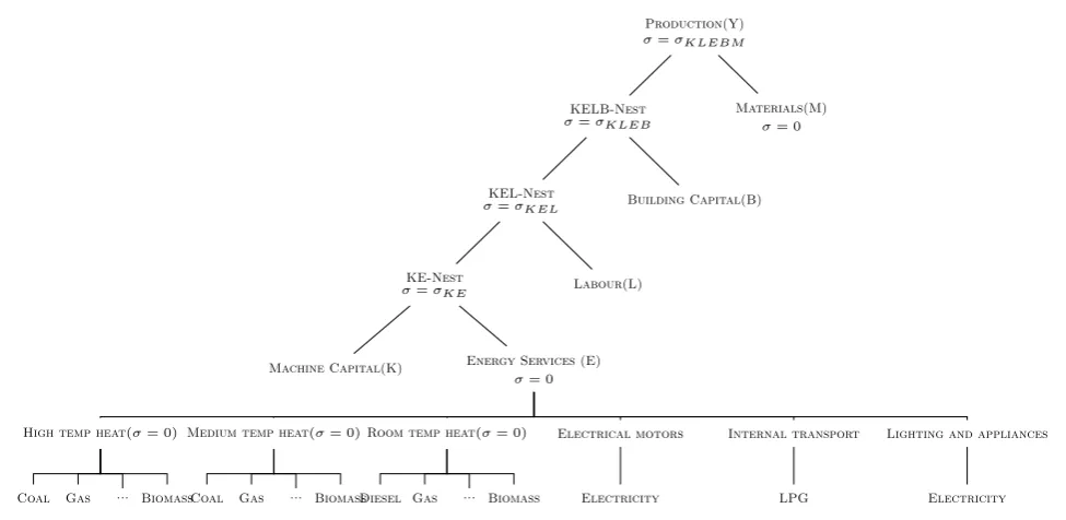
Figure 2: CGE nesting structure

Production(Y) σ=σ_KLEBM

KELB-Nest σ=σ_KLEB

KEL-Nest σ=σ_KEL

KE-Nest σ=σ_KE

Machine Capital(K) Energy Services (E) σ= 0

High temp heat(σ= 0)

Coal Gas ... Biomass

Medium temp heat(σ= 0)

Coal Gas ... Biomass

Room temp heat(σ= 0)

Diesel Gas ... Biomass

Electrical motors

Electricity

Internal transport

LPG

Lighting and appliances

Electricity Labour(L)

Building Capital(B) Materials(M)

σ= 0

parameters in traditional CGE models.

4.2. Capturing the activity and the price effects

Within IntERACT, we rely on the CGE model to determine the activity and price effects for the ten final energy using industrial sectors. Armington elasticities are used to model trade, i.e., foreign goods are imperfect substitutes for domestically produced (Armington, 1969). The model consists of the following factor markets: labor, machinery capital, and building capital. Labor and capital markets are homogeneous and mobile (aside from the capital tied to energy service capacity). These properties, combined with the absence of price rigidity, make the model relevant as a long-term perspective. Two components determine the activity effect within the CGE model: i) the baseline GDP calibration, and; ii) the relative change in sectoral activity. For the baseline scenario, we calibrate the GDP growth rate in the CGE model to match the exogenous baseline path by adjusting a Hicks-neutral technology innovation index (Barro and Sala-I-Martin, 1995). The level of investments, foreign trade balance, as well as public sector activity, are fixed for each modeling year based on the same exogenous macroeconomic baseline. Hence, the baseline reflects a consistent long term projection for the Danish Economy. When using IntERACT for a policy scenario, we fix the Hicks-neutral technology innovation index at its baseline scenario level, which means that GDP becomes endogenous in the policy scenario.

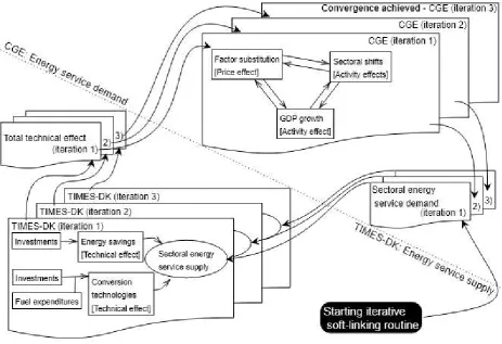
Figure 3: Capturing price, activity and technical effects in IntERACT

changes in the relative input price or changes in sectoral activity. The CGE model captures the price effect associated with input substitution in the sectoral production function, which is driven by the change in relative input prices. Figure 2 illustrates the generic production structure of the ten industrial sectors in the CGE model. Each node in the figure represents a constant elasticity of substitution function with a particular substitution elasticity2

. All industrial sectors are modeled using a standard constant elasticity of substitution (CES) function.

4.3. Consolidating the interaction effects

Figure 3 illustrates how the iterative soft-linking routine allows us to capture the three effects as well as the interaction effect. The figure is divided diagonally using a dotted line. Below the dotted line, TIMES-DK determines the energy service supply. Above the line, the CGE model determines the energy service demand.

We start the iterative routine by running TIMES-DK based on exogenous sectoral de-mand for energy services. Running TIMES-DK determines the primary technical effect in

2_{A separate study has guided the choice of nesting structure and substitution elasticities (Thomsen,}

terms of investment and fuel expenditures associated with energy savings and conversion technologies (bottom left of figure 3). Based on the technical effect from TIMES-DK, we update energy service prices and energy service production technology (including capital usage) for each industry and each energy service in the CGE model for future years. The CGE model determines the activity and price effects simultaneously (upper right of figure 3), based on the primary technical effect from TIMES-DK. The resulting future energy service demand from the CGE model is then fed back into TIMES-DK to capture second-round technical interaction effects. After 3–5 such iterations, we observe convergence between TIMES-DK and the CGE model. We use the absolute convergence between fuel costs and tax revenues (for each sector and energy service) as convergence criterion. We also observe convergence in capital cost for each energy service between the CGE model and TIMES-DK, although not absolute convergence due to the conceptual differences between the CGE model and TIMES-DK when it comes to capital demand (Andersen et al., 2019).

Table 2: Primary and interaction effects of modelling components on energy service demand in IntERACT

IntERACT component Primary effect Interaction effects Model

1. GDP growth (a) CGE

2. Sectoral change (a) (b,c) CGE

3. Factor substitution (b) (a,c) CGE

4. Energy savings (c) (b,a) TIMES-DK

5. Conversion technology (c) (b,a) TIMES-DK

(a) Activity effect; (b) Price effect; and (c) Technical effect

Table 2 showcase the five components in the IntERACT model, which constitute the activity, price, and technical effects. Table 2 further highlight both the primary effect and secondary interaction effects for each component. Calibrating GDP-growth using a Hicks-neutral technology innovation index only results in activity effect (a_{); i.e., no interaction}

effect. Since this type of calibration corresponds to a simple scaling of (the constant returns to scale) economy. The activity effect from sectoral shifts (associated with the baseline cal-ibration or policy scenarios) may well result in additional interaction effects. These occur if sectoral shifts affect relative prices within the economy (price effect) or if sectoral shifts lead to additional investment in energy service production (technical effect). The price effect (b₎

which is driven by factor input substitution may lead to interaction effects if a higher price of capital reduces competitiveness and, thereby, activity in a sector, or if the price of capi-tal changes the demand for energy services within a sector; leading to secondary technical effects. The technical effect (c_{), driven by the investment in energy savings and}

5. Results and discussion

This section demonstrates how IntERACT allows us to conduct an ex-ante evaluation of an energy efficiency policy. For this purpose, we consider a baseline (without energy efficiency policy) and an energy efficiency policy scenario.

For each scenario, we solve the IntERACT model until the year 2050. However, this section focuses on the policy impact in the year 2030. This choice reflects the contemporary policy focus within EU member states on meeting energy savings obligations under the Energy Efficiency Directive for the period 2021 to 2030 (European Union, 2018).

We decompose the change in final energy use between 2015 and 2030 for the baseline and policy scenarios. We rely on an adapted version of the shift-share decomposition technique; following Dunn Jr (1960)3_.

Using this decomposition technique, we highlight how the additional energy savings from the energy efficiency policy is composed of opposing technical, price, and activity effects. We compare the size of the rebound effects with the literature reviewed in section 3. Finally, we discuss the modeling of the policies that reduce the energy efficiency gap.

5.1. Baseline scenario

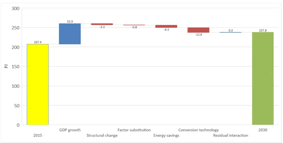
The comprehensiveness of the IntERACT model makes it possible to decompose the baseline scenario in terms of final energy use changes, which are driven by activity, price, and technical effects. Figure 4 decomposes the change in total industry final energy use between 2015 and 2030 for the baseline scenario. Final energy use increases by 30.4 PJ to 237.8 PJ in 2030. GDP growth is the most important driver behind the increase in energy use during the period. On its own, GDP growth would increase the total final energy use by 52.9 PJ. The change in the relative activity of sectors reduces final energy use by 3.2 PJ during the period, which reflects the underlying trend that non-energy intensive sectors grow relatively more than energy-intensive sectors; a result that is in line with the historical trend in Denmark. Together, the growth and structural effects make up the activity effect component. The decomposition further reveals a small reduction in energy use due to factor substitution, or price effect (-0.8 PJ). The combined technical effect results in a reduction in the final energy use of 18.9 PJ. Investments in new conversion technologies reduce final energy use by 12.6 PJ, whereas energy savings contribute to a reduction in final energy use of 6.3 PJ. Finally, the decomposition methodology captures a minor residual interaction effect (0.3 PJ), which we cannot readily attribute to any of the three effects.

5.2. Capturing the additionality of energy efficiency policy

Accounting for the baseline allows us to evaluate the additionality associated with an energy efficiency policy scenario. To this end, we consider a policy scenario that includes

3_{This is basically a structural decomposition analysis that allows us to decompose changes in, e.g., energy}

Figure 4: Decomposing change in baseline scenario final energy use between 2015 and 2030

Note: Final energy use in this figure includes solar heating and ambient heat used in heat pump

both an up-front investment subsidy (around 0.01 Euros per kWh saved over the lifetime of the savings measure) and policies that address the energy efficiency gap by reducing the investment barriers associated with energy-saving measures. We model the reduction in investment barriers as a reduction in the hurdle rate from 20% to 11% for industry energy-saving measures.

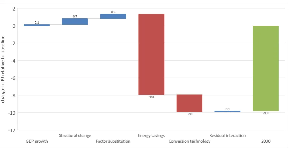
Section 5.2 discusses the choice of hurdle rate and its effect on the additionality in detail. Figure 5 captures the net impact of the industrial energy efficiency policy in terms of change in total final energy and change in each component relative to the baseline scenario. The energy efficiency policy results in a reduction of 9.8 PJ in final energy use in 2030 compared to the baseline scenario. However, this additionality is the product of opposing technical, activity, and price effects. The energy efficiency policy increases energy savings by 9.3 PJ relative to the baseline. Furthermore, it leads to a reduction of 2 PJ in final energy use from conversion technologies, which reflects how investments in energy savings reduce reliance on the most expensive and energy inefficient conversion technologies. The energy efficiency policy results in the avoidance of 2.5 million tonnes of cumulative CO2-emissions

for the period 2018–2030 relative to the baseline scenario4_.

The change in growth, structural, and factor substitution effects captures the total re-bound associated with the energy efficiency policy, which amounts to 1.3 PJ. The growth effect (which reflects the economy-wide rebound) is very small, albeit with a positive sign,

4_{corresponding to around 7.2% of total annual Danish CO}

2-emissions from energy use in 2017 (Danish

Figure 5: Decomposing policy impact from industry energy efficiency scenario in 2030 relative to baseline)

Note: Final energy use in this figure includes solar heating and ambient heat used in heat pump

reflecting a minor positive impact from the energy efficiency policy on GDP. The structural effect (indirect rebound effect) is 0.7 PJ, i.e., the energy efficiency policy leads to a slight increase in the relative activity of the energy-intensive sectors. The price effect (reflecting the price-induced rebound effect) leads to additional demand compared to the baseline of 0.5 PJ as energy services become relatively cheaper compared to other factors. Finally, we also observe a minor increase in final energy use associated with the residual interaction effect of 0.1 PJ.

5.3. Additional savings derived from reducing the energy efficiency gap

In the baseline scenario, we assume that several internal barriers exist at the firm level, which results in a substantial energy efficiency gap. These barriers include a lack of access to capital, information, and skills as well as barriers associated with the complex decision chains within industries. We use the 20 % hurdle rate to represent the energy savings investment behavior of firms associated with the baseline energy efficiency gap.

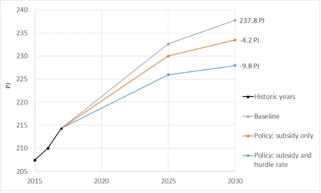
Figure 6: Impact assessment of reducing barriers to energy savings investment

research as it may well depend on the national policy context in particular; both in terms of existing policy measures and the additional policy measure under consideration. In a study focusing on the industrial sector in the USA, Qiu et al. (2015) find that increasing energy efficiency policy pressure in the form of recommended energy-saving measures lowers the implied discount rate (or hurdle rate) by around nine percentage points. Inspired by Qiu et al. (2015), this paper assumes that the energy efficiency policy reduces barriers to investments in energy efficiency corresponding to a hurdle rate reduction from 20 % to 11 %. Figure 6 highlights the importance of the assumed hurdle rate reduction; by comparing the final energy use in (i) the baseline scenario, (ii) a subsidy-only policy scenario, and (iii) the policy scenario which includes both the subsidy and hurdle rate reduction. Excluding the hurdle rate reduction from the policy scenario, reduces the additionality down from 9.8 PJ to 4.2 PJ. Hence reducing the energy efficiency gap accounts for more than half of the additional energy savings within the policy scenario.

This result underscores the importance of the energy efficiency gap for ex-ante energy efficiency assessments and emphasizes the need for more research into the choice of industry hurdle rates. However, Figure 6 demonstrates how a model like IntERACT (unlike ) allows us to explicitly evaluate the impact of the energy efficiency gap on the policy outcome; a vital improvement compared to the standard top-down modeling approach.

5.4. The rebound effects from the energy efficiency policy

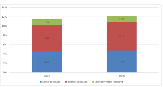
Figure 7: Rebound effects in the policy scenario in 2025 and 2030

In line with Hanley et al. (2006), we find that the activity effects (the sum of the indirect and economy-wide rebound) dominate the price effect (direct rebound). The indirect re-bound represents the largest relative rere-bound effect, increasing from 5.6 % in 2025 to 6.2 % in 2030 (cf. Figure 7). The second-largest effect is the direct rebound associated with the policy scenario, which increases from 4.5 % to 5.2 %. Finally, the economy-wide rebound remains relatively constant over the periods constituting 1.3 % of the technical effect. We note that the size of the indirect and economy-wide rebound depends critically on the choice of Armington elasticities. Halving the assumed Armington elasticities (from four to two) also halves the indirect and economy-wide rebound associated with the policy scenario. The size of the indirect rebound and economy-wide rebound further reflects two key modeling assumptions, which may work in opposite directions. First, the assumption that capital is homogeneous in IntERACT may lead to an overestimation of the indirect rebound as capital and labor are free to reallocate across sectors. Including barriers to capital mobility, would likely reduce the indirect rebound effect. Second, the fact that we do not solve the CGE model by using intertemporal optimization probably reduces both the economy-wide and indirect rebound within the model as the capital stock cannot adjust following a change in capital demand. Therefore, future research should focus on modeling barriers to capital mobility and intertemporal investment and savings behavior.

For energy-intensive sectors, the total rebound is around 23 % (ranging from 13–34 %), while the effect for non-energy-intensive sectors is around 4 % (ranging from 2–7 %). Overall, these results confirm previous findings by Barker et al. (2007a,b), who calculate the rebound effect for energy-intensive industries to be between 20–30 %, and between 5–10 % for non-energy intensive sectors. However, Barker et al. (2007b) find an overall total rebound effect of around 26 %, which is significantly larger than the 12 % we calculate here (cf. Figure 7). The differences in sectoral structure between the UK and Denmark may play a role in explaining this difference.

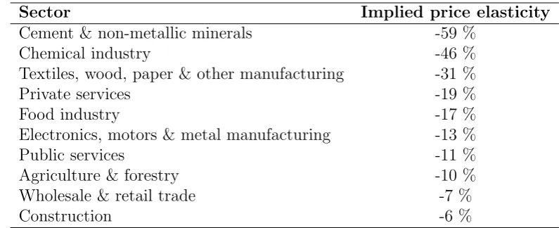
reduction in final energy use in 2030 relative to the baseline scenario, energy service costs are only reduced by 1.4 % on average across sectors. This result reflects how the technical effect shifts energy service production technology towards being more capital intensive and less dependent on energy inputs. As such, the direct rebound effect reflects the average implicit price elasticity of around -16 %. Table 3 highlights the implicit price elasticities at the sectoral level. Not surprisingly, we see that energy-intensive sectors, such as cement and chemical industries, have higher implicit price elasticities than non-intensive sectors, such as wholesale & retail trade. In general, energy costs tend to make up a larger share of the value of production or output from energy-intensive sectors, which also contributes to higher implicit price elasticity. Furthermore, the estimated production system reveals higher elasticities of substitution between energy and capital for energy-intensive sectors with high energy cost shares.

Table 3: Average implied own-price elasticities of energy service demand by sector in 2030

Sector Implied price elasticity

Cement & non-metallic minerals -59 %

Chemical industry -46 %

Textiles, wood, paper & other manufacturing -31 %

Private services -19 %

Food industry -17 %

Electronics, motors & metal manufacturing -13 %

Public services -11 %

Agriculture & forestry -10 %

Wholesale & retail trade -7 %

Construction -6 %

6. Conclusion

The industry energy efficiency policy considered in this paper results in the avoidance of 2.5 million tonnes of cumulative industrial CO2-emissions during the period 2018–2030.

This level of avoidance corresponds to roughly 5% of Danish greenhouse gas emissions in 2016, underscoring the importance of energy efficiency as a tool for reducing greenhouse gas emissions.

and the increases in the energy efficiency of conversion technology. Conversely, the price effect (direct rebound) increases final energy use by 0.5 PJ, and the activity effect (indirect and economy-wide rebound) increases demand by 0.8 PJ. The decomposition shows the importance of including all three effects when assessing the net effect of an energy efficiency policy for industrial sectors. The paper has further demonstrated how the size of the price and activity effects varies greatly by sectors.

Previous studies have sought to capture these effects, but none have been able to combine all three effects simultaneously while accounting for the interaction between them. Hence the IntERACT modeling approach demonstrated in this paper represents a significant leap forward in terms of performing a comprehensive ex-ante evaluation of energy efficiency policy for industrial sectors.

7. Acknowledgements

We are grateful for the financial support of the Danish Energy Agency and Innovation Fund Denmark under the research project SAVE-E, grant no. 4106-00009B. We are solely responsible for any errors or omissions. We note that the views expressed in this paper are those of the authors and not necessarily those of the Danish Energy Agency.

8. Reference

Allan, G., Hanley, N., Mcgregor, P., Swales, K., Turner, K., 2007. The impact of increased efficiency in the industrial use of energy: A computable general equilibrium analysis for the United Kingdom. Energy Economics 29, 779–798, doi:10.1016/j.eneco.2006.12.006.

Andersen, K.S., Termansen, L.B., Gargiulo, M., ´O Gallach´oirc, B.P., 2019. Bridging the gap using energy services: Demonstrating a novel framework for soft linking top-down and bottom-up models. Energy 169, 277–293.

Armington, P.S., 1969. A Theory of Demand for Products Distinguished by Place of Production. Interna-tional Monetary Fund Staff Papers XVI, 159–78.

Balyk, O., Andersen, K.S., Dockweiler, S., Gargiulo, M., Karlsson, K., Næraa, R., Petrovi´c, S., Tattini, J., Termansen, L.B., Venturini, G., 2019. TIMES-DK: Technology-rich multi-sectoral optimisation model of the Danish energy system. Energy Strategy Reviews 23, 13–22.

Barker, T., Dagoumas, A., Rubin, J., 2009. The macroeconomic rebound effect and the world economy. Energy Efficiency 2, 411–427, doi:10.1007/s12053-009-9053-y,arXiv:0402594v3.

Barker, T., Ekins, P., Foxon, T., 2007a. Macroeconomic effects of efficiency policies for energy-intensive industries: The case of the UK Climate Change Agreements. Energy Economics 29, 760–778, doi:10.1016/j.eneco.2006.12.008.

Barker, T., Ekins, P., Foxon, T., 2007b. The macro-economic rebound effect and the UK economy. Energy Policy 35, 4935–4946, doi:10.1016/j.enpol.2007.04.009.

Barro, R.J., Sala-I-Martin, X., 1995. Economic Growth. Interation ed., McGraw-Hill Book Co.

Bataille, C., Jaccard, M., Nyboer, J., Rivers, N., 2006. Towards General Equilibrium in a Technology-Rich Model with Empirically Estimated Behavioral Parameters. Energy Journal .

Bataille, C., Melton, N., 2017. Energy efficiency and economic growth: A retrospective CGE analysis for Canada from 2002 to 2012. Energy Economics 64, 118–130, doi:10.1016/j.eneco.2017.03.008.

Berndt, E.R., 1990. Energy use, technical progress and productivity growth: A survey of economic issues. Journal of Productivity Analysis 2, 67–83, doi:10.1007/BF00158709.

Danish Energy Agency, 2018. Energy statistics 2017. Danish Energy Agency, Copenhagen, Denmark. Danish Energy Agency, Energinet, 2016. Technology Data for Individual Heating Installations. Technical

Report August 2016. Danish Energy Agency & Energinet.

DEA, 1995. Teknologikatalog energibesparelser i erhvervslivet - ”technology catalogue - energy savings in industry” (freely translated). Danish Energy Agency .

Dunn Jr, E.S., 1960. A statistical and analytical technique for regional analysis. Papers in Regional Science 6, 97–112.

European Union, 2018. Directive (EU) 2018/2002 of the European Parliament and of the Council of 11 De-cember 2018 amending Directive 2012/27/EU on energy efficiency (Text with EEA relevance.). Technical Report. European Union.

Filippini, M., Hunt, L.C., 2015. Measurement of energy efficiency based on economic foundations. Energy Economics 52, S5–S16, doi:10.1016/j.eneco.2015.08.023.

Goldberg, M.L., Barry, J.R., Dunn, B., Ackley, M., Robinson, J., Deangelo-Woolsey, D., 2011. Focus on Energy Evaluation. Business Programs: Measure Life Study. Technical Report. PA Consulting Group Inc. for State of Wisconsin Public Service Commission of Wisconsin.

Greening, L.a., Greene, D.L., Difiglio, C., 2000. Energy effciency and consumption - the rebound effect - a survey. Energy Policy 28, 389–401, doi:10.1016/S0301-4215(00)00021-5.

Grepperud, S., Rasmussen, I., 2004. A general equilibrium assessment of rebound effects. Energy Economics 26, 261–282, doi:10.1016/j.eneco.2003.11.003.

Grifell-Tatj´e, E., Lovell, C.A., 2000. Cost and productivity. Managerial and Decision Economics 21, 19–30, doi:10.1002/1099-1468(200001/02)21:1¡19::AID-MDE962¿3.0.CO;2-7.

Hanley, N.D., McGregor, P.G., Swales, J.K., Turner, K., 2006. The impact of a stimulus to energy efficiency on the economy and the environment: A regional computable general equilibrium analysis, in: Renewable Energy, pp. 161–171, doi:10.1016/j.renene.2005.08.023.

Hartwig, J., Kockat, J., Schade, W., Braungardt, S., 2017. The macroeconomic effects of ambitious energy efficiency policy in Germany Combining bottom-up energy modelling with a non-equilibrium macroeco-nomic model. Energy 124, 510–520, doi:10.1016/j.energy.2017.02.077.

Hoffman, I.M., Schiller, S.R., Todd, A., Billingsley, M.A., Goldman, C.A., Schwartz, L.C., 2015. Energy Savings Lifetimes and Persistence: Practices, Issues and Data. Technical Report May. Lawrence Berkeley National Lab (LBNL). Berkeley, California, United States.

Hunt, L.C., Ryan, D.L., 2015. Economic modelling of energy services: Rectifying misspecified energy demand functions. Energy Economics 50, 273–285, doi:10.1016/j.eneco.2015.05.006.

Huntington, H.G., 1994. Been top down so long it looks like bottom up to me. Energy Policy 22, 833–839, doi:10.1016/0301-4215(94)90142-2.

IEA, 2017. Energy Technology Perspectives 2017. OECD,arXiv:© OECD&IEA, 2014.

Johanson, M., Petersen, P.M., 2009. Energibesparelser i erhvervslivet - ”energy savings in industry” (freely translated). Report for the Danish Energy Agency DGC by Dansk Energi Analyse A/S Viegand Maage ApS. .

Koopmans, C.C., Te Velde, D.W., 2001. Bridging the energy efficiency gap: Using bottom-up information in a top-down energy demand model. Energy Economics 23, 57–75, doi:10.1016/S0140-9883(00)00054-2. Kromann, M., Kragerup, H., Dalsgaard, M., Carsten, K., Godkendt, G., 2015. Kortlægning af

energispare-potentialer i erhvervslivet (in Danish). Technical Report. COWI / Danish Energy Agency.

Loulou, R., Goldstein, G., Kanudia, A., Lettila, A., Remme, U., 2016. Documentation for the TIMES Model. Technical Report July. Energy Technology Systems Analysis Programme.

McKinsey, 2007, . Reducing US greenhouse gas emissions: how much at what cost?: US Greenhouse Gas Abatement Mapping Initiative.

McNeil, M.A., Letschert, V.E., de la Rue du Can, S., Ke, J., 2013. Bottom-Up Energy Analysis System (BUENAS)-an international appliance efficiency policy tool. Energy Efficiency 6, 191–217, doi:10.1007/s12053-012-9182-6.

Murphy, R., Jaccard, M., 2011. Energy efficiency and the cost of GHG abatement: A comparison of bottom-up and hybrid models for the US. Energy Policy 39, 7146–7155, doi:10.1016/j.enpol.2011.08.033. Official Journal of the European Communities, 2009. Directive 2009/125/ec of the european parliament and

of the council of 21 october 2009, establishing a framework for the setting of ecodesign requirements for energy related products. Official Journal of the European Communities .

Official Journal of the European Communities, 2017. Regulation (eu) 2017/1369 of the european parlia-ment and of the council of 4 july 2017 setting a framework for energy labelling and repealing directive 2010/30/eu. Official Journal of the European Communities .

Oxera, A., 2011. Discount rates for low-carbon and renewable generation technologies. Report. Oxera Consulting LLP .

Qiu, Y., Wang, Y.D., Wang, J., 2015. Implied discount rate and payback threshold of energy efficiency investment in the industrial sector. Applied Economics 47, 2218–2233.

Rosenow, J., Pat´o, Z., Fawcett, T., 2016. An exante evaluation of the EU Energy Efficiency Directive -Article 7. Economics of Energy & Environmental Policy 5.

Sorrell, S., 2009. Jevons’ Paradox revisited: The evidence for backfire from improved energy efficiency. Energy Policy 37, 1456–1469, doi:10.1016/j.enpol.2008.12.003.

Sorrell, S., Mallett, A., Nye, S., 2011. Barriers to industrial energy efficiency: A literature review . Thomsen, T., 2015. KLEM-estimationer (in Danish).

Vine, E., 2008. Breaking down the silos: The integration of energy efficiency, renewable energy, demand response and climate change, doi:10.1007/s12053-008-9004-z.

Appendix A: Methodology for decomposing IntERACT results

This appendix explains the methodology used for decomposing results from the IntER-ACT model. The objective is to decompose the change in final energy use from one period to another into several components: growth effect, structural change effect, factor substitu-tion effect, energy savings effect, and a conversion technology effect. We decompose starting with the use of the shift-share technique, based loosely on Dunn Jr (1960). First, we look at final energy use across different sectors, defining the change in energy use by either growth in production, structural shifts between sectors or efficiency changes. This decomposition reveals the activity effect as the sum of the structural and growth components. The remain-ing efficiency component comprises of several effects. We decompose this component into three sub-components explaining changes to energy efficiency: relative factor substitution effect, energy savings effect, and conversion technology effect. From this, we can define the price effect as the relative factor substitution effect, and the technical effect as the sum of the energy savings and conversion technology effects.

We apply the following definitions:

E ₌X

i

E_i Y ₌X

i

Y_i s_{i =} Yi Y e=

E

Y ei = E_i Y_i

Here, E _{is final energy use,} Y _{is the production value,} e _{is energy intensity,} s _{is share}

and i _{is sector.}

We write the intensity as the weighted sum of all sectors’ intensities:

e₌ E Y

=X

i

E_i Y

=X

i

E_i Y

Y_i Y_i

=X

i

E_i Y_i

Y_i Y

=X

i

e_is_i

=X

i

(e_{i+ ¯}e_i−e¯_i)(s_i+ ¯s_i−s¯_i)

(1)

e−e¯=

X

i

(e_{i+ ¯}e_i−e¯_i)(s_i+ ¯s_i−s¯_i)−

X

i ¯

e_is_¯i

=X

i

e_is_i+X

i

e_is_¯i−X

i

e_is_¯i+X

i ¯

e_is_i+X

i ¯

e_is_¯i−

X

i ¯

e_is_¯i−X

i ¯

e_is_i−X

i ¯

e_is_¯i+X

i ¯

e_is_¯i−X

i ¯

e_is_¯i

=X

i ¯

e_i(s_i−s¯_i) +

X

i

(e_i−e¯_i) ¯s_i+

X

i

(e_i−e¯_i)(s_i−s¯_i)

(2)

Using equation 2, we can decompose changes in energy intensity e _{in a structural term;}

P

ie¯i(si−s¯i), an efficiency term; P

i(ei−e¯i) ¯si, and an interaction effect between the two; P

i(ei−e¯i)(si−s¯i). Moving to decompose changes to final energy consumption (E −E¯) instead of intensities, we rewrite equation 2 so thatE ₌Y e_:

E−E¯ =Y e−Y¯¯e

=Y₍e_{+ ¯}e−e¯)−Y¯e¯

=Y₍e−e¯) + (Y −Y¯)¯e

=Y X

i ¯

e_i(s_i−s¯_i) +Y

X

i

(e_i−e¯_i) ¯s_i+

Y X

i

(e_i−e¯_i)(s_i−s¯_i) + (Y −Y¯)¯e

(3)

Therefore, equation 3 makes it possible to decompose changes in final energy consumption into the following 4 components:

1. A growth component, where sectoral structure and intensities are held constant. (Y −Y¯)¯e

2. A structural component, where intensities are held constant. Y P

ie¯i(si−s¯i) 3. An efficiency term, where sectoral structure is held constant. Y P

i(ei−e¯i) ¯si 4. An interaction effect. Y P

i(ei−e¯i)(si−s¯i)

As noted earlier, we now have obtained the activity effect (the sum of the growth and structural effects). Further decomposition is required to be able to distinguish the price and technical effects, both components of the efficiency effect. To achieve this, we decompose the efficiency term of equation 3 into the following three sub-components: a factor substitution effect, an energy savings effect, and a conversion technology effect. More sub-components might contribute to the efficiency effect, but are neglected here.

substitution effect towards factors other than energy services, and as a result, energy use will decline. Thus, FSE changes to energy use because of relative factor substitution. We apply the following definition:

ES_{i =}X

s

E_i,s∗C_i,s

WhereES_{iis the energy service demand per sector,}i_{, summed over all energy services,}s_,

defining ES_{i in terms of useful energy, or net energy.} C_{i,s is the conversion loss or efficiency}

of conversion technologies per sector, i_{, and energy service,} s_.

Equation 4 shows how factor substitution effect is defined in terms of final energy.

F SE ₌X

i

ES_i−ES_i

ES_i

−

Y_i−Y¯_i

¯

Y_i

ES_i Ei ES_i

(4)

Thus, summed over all sectors, the first part of equation 4 calculates the difference in the growth of energy service demand and production output. We convert this to absolute changes to energy service demands by multiplying with the sum of energy service demands by sector. Since we define energy service demand in terms of useful energy, we convert into final energy using the fuel intensity of energy service production.

Finding the energy-saving effect is straightforward when using the TIMES-DK model as we read out the number of energy services provided by energy-saving investments. As noted earlier, energy savings can take the form of equipment, such as retrofitting and insulation, and management, such as process route optimization. Equation 5 shows how the energy-saving effect in terms of final energy.

ESAV ₌X

i,s

SAV_i,s Ei,s ES_i,s

(5)

Thus, per sector, i_{, and energy service,} s_{, we convert energy savings,} SAV _{in terms of}

useful energy to final energy using fuel intensity of energy service production.

We term the remaining residual from the energy efficiency component from equation 3 the conversion technology effect (CTE). This residual captures conversion technology im-provements, and fuel switching. We calculate this effect in equation 6:

Y X

i

(e_i−e¯_i)s_i =F SE−ESAV −CT E ⇔

CT E₌Y X

i

(e_i−e¯_i)s_i−F SE−ESAV

Now we have further decomposed changes in final energy use, following equation 3:

E−E¯ =Y X

i ¯

e_i(s_i−s¯_i) +Y X

i

(e_i−e¯_i) ¯s_i+

Y X

i

(e_i−e¯_i)(s_i−s¯_i) + (Y −Y¯)¯e ⇔

E−E¯ =Y

X

i ¯

e_i(s_i−s¯_i) +

X

i

ES_i−ES_i

ES_i

−

Y_i−Y¯_i

¯

Y_i

ES_i Ei ES_i

+

X

i,s

SAV_i,s Ei,s ES_i,s

+

Y X

i

(e_i−e¯_i)s_i−F SE−ESAV+

Y X

i

(e_i −e¯_i)(s_i−s¯_i) +

(Y −Y¯)¯e

(7)

Thus,, equation 7 yields the five components that attribute the three main effects (i.e., the activity, price, and technical effect).

• Activity effect, which consists of a:

– Growth effect component, defined in equation 3:

(Y −Y¯)¯e

– Structural effect component, defined in equation 3:

Y P

ie¯i(si−s¯i)

• Price effect, which consists of a:

– Factor substitution effect, defined in equation 4:

F SE ₌P i

ESi−ESi ESi

− Yi−_¯Y¯i

Yi

ES_i Ei ESi

• Technical effect, which consists of a:

– Energy savings effect, defined in equation 5:

ESAV ₌P

i,sSAVi,s _E

i,s ESi,s

– Conversion technology effect, defined in equation 6:

CT E ₌Y P

• Residual effect, which consists of a:

– Interaction effect, defined in equation 3:

Y P