Munich Personal RePEc Archive
Partial effects estimation for fixed-effects
logit panel data models
Bartolucci, Francesco and Pigini, Claudia
18 February 2019
Online at
https://mpra.ub.uni-muenchen.de/92251/
Partial effects estimation for fixed-effects
logit panel data models
Francesco Bartolucci
Universit`a di Perugia (IT) [email protected]
Claudia Pigini
Universit`a Politecnica delle Marche and MoFiR (IT)
Abstract
We propose a multiple step procedure to estimate Average Partial Effects (APE) in fixed-effects panel logit models. Because the incidental parameters problem plagues the APEs via both the inconsistent estimates of the slope and individ-ual parameters, we reduce the bias by evaluating the APEs at a fixed-T consistent estimator for the slope coefficients and at a bias corrected estimator for the unob-served heterogeneity. The proposed estimator has bias of order O(T−2
) asn→ ∞
and performs well in finite sample, even when nis much larger than T. We provide a real data application based on the labor supply of married women.
Keywords: Average partial effects, Bias reduction, Binary panel data, Conditional Maximum Likelihood
1
Introduction
Practitioners who estimate binary choice models are often interested in quantifying the effect of some regressorxon the response probability, other things being equal. Moreover, with the availability of panel data, the fixed-effects approach allows for the estimation of partial effects of covariates that may be correlated with the individual specific unobserved heterogeneity in a nonparametric manner.
The Maximum Likelihood (ML) estimator of fixed-effects binary choice models, how-ever, is consistent only as T → ∞ and otherwise suffers form the well-known incidental parameters problem (Neyman and Scott, 1948; Lancaster, 2000).1 With fixed T, the
plug-in estimator of the Average Partial Effect (APE) of some covariate on the response probability is also plagued by the incidental parameters problem, which gives rise to two sources of bias: one is introduced by the ML estimator of the individual effects, consistent only as T → ∞; the other is carried over by the ML estimates of the slope parameters, that are affected by the bias in the estimated subject-specific intercepts as they are not informationally orthogonal.
We propose a multiple step procedure to estimate the APE in fixed-effects panel logit models with a reduced order of bias. The bias introduced by the estimated slopes is removed by using the fixed-T consistent Conditional Maximum Likelihood (CML) esti-mator for parameters of the fixed-effects logit model, for which the incidental parameters problem can be solved by conditioning on simple sufficient statistics for the individual intercepts (Andersen, 1970; Chamberlain, 1980). The bias that comes with the ML es-timates of the individual intercepts is reduced from O(T−1
) to O(T−2
) by defining the ML estimator for the individual unobserved heterogeneity as the solution to the modified score function put forward by Firth (1993).
The proposed procedure, however, cannot be extended directly to the dynamic logit (Hsiao, 2005), for which CML inference for the slope parameters is not viable in a simple form. This is overcome by Bartolucci and Nigro (2010), who propose a Quadratic Ex-ponential (QE) formulation (Cox, 1972) to model dynamic binary panel data, that has the advantage of admitting sufficient statistics for the individual intercepts. Furthermore, Bartolucci and Nigro (2012) propose a QE model, that approximates more closely the dynamic logit model, the parameters of which can easily be estimated by Pseudo CML (PCML). We therefore extend the proposed procedure to include PCML estimates in the APEs when a dynamic logit is specified.
Several contributions deal with bias reduction techniques for the ML estimators of fixed-effects binary choice models. Some of them provide bias corrections for the APEs as well, along the same lines of the corrections proposed for the slopes. Analytical corrections
1
We focus on large n and largeT perspective, as APEs are often not point identified with fixed T
are provided by Fern´andez-Val (2009), whose derivations are based on general results for static (Hahn and Newey, 2004) and dynamic (Hahn and Kuersteiner, 2011) nonlinear panel data models. An alternative bias correction method for the APE estimator relies on the panel jackknife. A general procedure for nonlinear static panel data models is proposed by Hahn and Newey (2004), whereas a split-panel jackknife estimator is developed by Dhaene and Jochmans (2015) for dynamic models.
As it happens with the proposed method, the analytical and jackknife corrections reduce the order of the bias for the APE from O(T−1
) to O(T−2
). However, these APE estimators depend on some bias corrected estimator for the slope coefficients which can be shown to have correct confidence intervals if T grows faster thann1/3 (Hahn and Newey,
2004). This is not required in our case. In fact, we show by simulation that the proposed APE estimator, although large-T consistent, performs well in finite samples even whenn
is much larger than T.
The rest of the paper is organized as follows: in Section 2 we briefly discuss the inciden-tal parameters problem and how it affects the APEs estimator; in Section 3 we illustrate the proposed methodology, its extension to accommodate the dynamic logit model, and briefly recall the alternative bias correction strategies; in Section 4 we investigate the fi-nite sample performance of the proposed estimator and compare it with that of the panel jackknife; in Section 5 we provide a real data application based on labor supply of married women. Finally, Section 6 concludes.
2
Average partial effects and the incidental
parame-ters problem
We consider n units, indexed with i = 1, . . . , n, observed at time occasions t = 1, . . . , T. Let yit be the binary response variable for unit i at occasion t and xit the corresponding vector of K covariates. We assume that bothyit and xit are independent across i and T. Consider the logit formulation
p(yit|xit;αi,β) =
exp [yit(αi+x′itβ)] 1 + exp(αi +x′itβ)
, (1)
where αi is the individual specific intercept, xit is vector of strictly exogenous covariates, and β collects the regression parameters.
by concentrating out the αi as the solution to
ˆ
β = arg max
β n X i=1 T X t=1
lnp(yit|xit; ˆαi(β),β),
ˆ
αi(β) = arg max αi
T
X
t=1
lnp(yit|xit;αi,β).
Notice that here ˆαi(β) depends on the data only through yi = (yi1, . . . , yiT)′ and Xi = (xi1, . . . ,xiT).
Because the estimation noise in ˆαi(β) disappears only asT → ∞, the ML estimator of ˆ
β is not consistent for β0 with T fixed and only n→ ∞, that is plim n→∞
ˆ
β≡βT 6=β0. This
is the well-known incidental parameters problem (Neyman and Scott, 1948; Lancaster, 2000). To clarify this, consider any function m(yi,Xi, αi) and let En[m(yi,Xi, αi)] ≡
lim n→∞
1
n
Pn
i=1m(yi,Xi, αi), where αi is treated as fixed. From standard extremum estima-tor properties, it follows that, with T fixed and as n→ ∞, βT is be obtained as
βT = arg max
β
En
" T X
t=1
lnp(yit|xit; ˆαi(β),β)
#
,
whereas β0 follows from
β0 = arg max
β
En
" T X
t=1
lnp(yit|xit;αi(β),β)
#
,
whereαi(β) maximizes ET [lnp(yit|xit;αi,β)]. From the expressions above it is clear that the problem arises from ˆαi(β)6=αi(β) with fixed T. Moreover, Hahn and Newey (2004) show that βT = β0 +B/T +O(T−2
). If, instead, T → ∞, then ˆαi(β) → αi0, with
αi0 = αi(β), and βT → β0. If both n, T → ∞, ˆβ will be consistent and asymptotically
normal. However, Hahn and Newey (2004) show that the asymptotic distribution of ML estimator will not be centered at its probability limit if n grows faster than T.
The incidental parameters problem severely affects the estimation of APEs as well, that are usually of interest to practitioners who want to quantify the effect of some regressor
x on the response probability, other things being equal. For the logit model in (1), the partial effect of covariate xitk for i at timet on the probability ofyit= 1 can be written, depending on the typology of covariate, as
mitk(αi,β,xit) =
p(yit = 1|αi,xit) [1−p(yit= 1|αi,xit)]βk, xitk continuous
p(yit = 1|αi,xit,−k, xitk = 1)−
where xit,−k denotes the subvector of all covariates but xitk. The true APE of the k-th
covariate can then be obtained by simply taking the expected value of fitk(αi,β,xit) with respect to xit:
µk0 ≡EnT [mitk(αi0,β0,xit)],
where µk0 ≡ µk(αi0,β0). An estimator of µk0 can be obtained by plugging in the ML
estimators ˆβ and ˆαi( ˆβ), so that
ˆ
µk = 1
nT
n
X
i=1
T
X
t=1
mitk(ˆαi( ˆβ),βˆ,xit). (2)
It is now clear that, with T fixed, this estimator is plagued by two sources of asymptotic bias: the first stems from the estimation error introduced by ˆαi(β), used instead of
αi(β); the second is a result of using the asymptotically biased estimator ˆβ. Dhaene and Jochmans (2015) show that the combined asymptotic bias is
plim n→∞
ˆ
µk =µk0+
D+E
T +O(T
−2
), (3)
where, specifically, Dis the bias the generates from using ˆαi(β) instead ofαi0, whereasE
is the bias from plugging in ˆβ, instead if usingβ0. Dhaene and Jochmans (2015) provide explicit expressions for D and E, based on the derivations by Fern´andez-Val (2009). Notice that, even if a fixed–T consistent estimator of β0 was available, the asymptotic bias of the APE estimator would still be of order O(T−1
) and equal to D/T.
3
Estimation of average partial effects
The previous section clarifies that a bias corrected estimators ofµk0 must take into account
the two sources of asymptotic bias combined in (3). In the following, we first illustrate the proposed methodology, which combines the consistent CML estimator of β0 and a bias corrected estimator of αi0. We then turn to the dynamic logit, for which the proposed
procedure is based on a PCML estimator. Finally, we briefly review the existing strategies with special attention to the jackknife procedure, that represent the benchmark against which to compare the finite sample performance of the proposed estimator.
3.1
Proposed methodology
The proposed two-step strategy is based on removing the two sources of bias in (3) by i) using the fixed-T consistent Conditional Maximum Likelihood (CML) estimator of β0, ˜β
instead of the ML estimator ˆβand ii) reducing the order of bias of ˆαi( ˜β) fromO(T−1) to
O(T−2
3.1.1 Two step estimation
The first step consists estimating by CML the structural parameters of the logit model in (1). Taking the the individual intercept αi as given, The joint probability of the response configuration yi = (yi1, . . . , yiT)′ conditional on Xi = (xi1, . . . ,xiT) can be written as
p(yi|Xi, αi) =
expyi+αi+PTt=1yitx′itβ
QT
t=11 + exp (αi+x
′
itβ)
.
It can be shown that the total scoreyi+ =Ptyit is a sufficient statistic for the individual interceptsαi (Andersen, 1970). The joint probability of yi = (yi1, . . . , yiT) conditional on
yi+ does not depend on αi and can therefore be written as
p(yi|Xi, yi+) =
exp
PT
t=1yitxit
′
β
P
z:z+=yi+
exp
PT
t=1ztxit
′
β
, (4)
where the denominator is the sum over all the response configurationz such thatz+=yi+
and where the individual interceptsαihave been canceled out. The log-likelihood function is
ℓ(β) = X i
I(0< yi+ < T) logp(yi|Xi, yi+),
where the indicator functionI(·) takes into account that observations with total scoreyi+
equal to 0 orT do not contribute to the log-likelihood andp(yi|Xi, yi+) is defined in (4).
The above function can be maximized with respect to βby a Newton-Raphson algorithm using standard results on the regular exponential family (Barndorff-Nielsen, 1978), so as to obtain the CML estimator ˜β, which is √n consistent and asymptotically normal with fixed–T (see Andersen, 1970; Chamberlain, 1980, for details). Therefore, if plugged into the APE formulation (2) instead of the ML estimator ˆβ, theE component of the bias in (3) is removed. Alternatively, Hahn and Newey (2004) suggest using a biased corrected version of ˆβfor which, however,T has to grow faster thannfor its asymptotic distribution to be centered at its probability limit.
The second step deals with obtaining estimates of the individual interceptsαi, which are not directly available as they have been canceled out by conditioning on the total score. One strategy would be to obtain the ML estimates of αi, for those subjects such that 0 < yi+ < T, by maximizing the individualPtlogpβ˜(yit|αi,xit) where pβ˜(yit|αi,xit) is the logit model probability in (1) evaluated at the CML estimateβ= ˜β. This strategy has been considered by Stammann et al. (2016). However, even if β is fixed at some
√
because ˆαi( ˜β) p
→αi0 only as T → ∞.
Our strategy is based on the proposal by Firth (1993), who shows that, for any ML estimator ˆψ with bias of order O(h−1
), where h is the number of observations, the score function U(ψ) can be modified as
U∗
(ψ) =U(ψ) + 1 2tr
I(ψ)−1∂I(ψ)
∂ψ′
,
whereI(ψ) is the Fisher Information matrix, so that the solution to the above estimating equation is an ML estimator with biasO(h−2
).2 We therefore obtain ˜αi( ˜β) as the solution
to
U∗
(αi) =U(αi) + 1 2I(αi)
∂I(αi)
∂αi =
T
X
t=1
(yit−˜rit) +
PT
t=1r˜it(1−r˜it)(1−2˜rit) 2hPT
t=1˜rit(1−r˜it)
i2 ,
where ˜rit= exp(αi+x′itβ˜)[1 + exp(αi+x′itβ˜)]. The resulting estimator of the individual intercept ˜αi will depend on ˜β, which we write as ˜αi( ˜β). The APEs can then be obtained by simply replacing the ML estimators in (2), that is
˜
µk = 1
nT
n
X
i=1
T
X
t=1
mitk(˜αi( ˜β),β˜,xit).
3.1.2 Standard errors
In order to derive an expression for the standard errors of the APEs ˜µ = (˜µ1, . . . ,µ˜K)′ we need to account for the use of the estimated parameters ˜β in the first step. We rely on the Generalized Method of Moments (GMM) approach by Hansen (1982) and also implemented by Bartolucci and Nigro (2012) for the Quadratic Exponential model. It consists in presenting the proposed multi-step procedure as the solution of the system of estimating equations
f(β,µ) =0,
where
f(β,µ) = n
X
i=1
I(0< yi+< T)fi(β,µ),
2
fi(β,µ) =
∇βℓi(β) ∇µ1gi(β, µ1)
...
∇µKgi(β, µK)
, (5) and
gi(β, µk) = 1
T
X
t
[mitk(αi(β),β,xit)−µk]2, k = 1, . . . , K.
The asymptotic variance of ( ˜β′,µ˜′
)′
is then
W( ˜β,µ˜) = H( ˜β,µ˜)−1
S( ˜β,µ˜)[H( ˜β,µ˜)−1
]′
, (6)
where
S( ˜β,µ˜) = X i
I(0< yi+ < T)fi( ˜β,µ˜)fi( ˜β,µ˜)
′
,
H( ˜β,µ˜) =X i
I(0< yi+< T)Hi( ˜β,µ˜),
and
Hi(β,µ) =
∇ββℓi(β) O ∇µβg
i(β,µ) ∇µµgi(β,µ)
, (7)
is the derivative of fi(β,µ) with respect to (β,µ), where O denotes a K×K matrix of zeros and gi(β,µ) collects gi(β, µk), for k = 1, . . . , K. Expressions for the derivatives in (5) are
∇βℓi(β) =
T
X
t=1
yitxit−
X
z:z+=yi+
p(z|Xi, yi+)
T
X
t=1
ztxit
!
,
and
∇µkgi(β, µk) =−
2
T
T
X
t=1
[mitk(αi(β),β,xit)−µk].
The second derivatives in (7) are
∇ββℓi(β) =
X
z:z+=yi+
p(z|Xi, yi+)e(z,Xi)e(z,Xi)
′
,
where
e(z,Xi) = T
X
t=1
ztxit−
X
z:z+=yi+
p(z|Xi, yi+)
T
X
t=1
ztxit
!
,
and∇µµg
i(β,µ) is aK×K diagonal matrix with element 2. Finally, for the computation of the block ∇µβgi(β,µ) we rely on numerical differentiation. Once the matrix in (6) is
3.1.3 The dynamic logit model
The method proposed to obtain the APE for the logit model cannot be applied directly to the dynamic logit (Hsiao, 2005). For the dynamic logit model, the conditional probability of yit being equal to 1 is
p(yit|xit, yi,t−1;ηi,δ, γ) =
exp [yit(ηi+xit′ δ+yi,t−1γ)]
1 + exp(ηi+x′itδ+yi,t−1γ)
, (8)
where γ is the regression coefficient for the lagged response variable that measures the true state dependence. Plugging the CML estimator of δ and γ in the APE formulation is not viable in this case because the total score is no longer a sufficient statistic for the incidental parameters if the lag of the dependent variable is included among the model covariates. Conditioning in sufficient statistics eliminates the incidental parameters only in the in the special case ofT = 3 and no other explanatory variables (Chamberlain, 1985). Honor´e and Kyriazidou (2000) extend this approach to include explanatory variables and parameters can be estimated by CML on the basis of a weighted conditional log-likelihood. However, time effects cannot be included in the model specification and the estimator’s rate of convergence to the true parameter value is slower than √n. This is overcome by Bartolucci and Nigro (2010), who propose a Quadratic Exponential (QE) formulation (Cox, 1972) to model dynamic binary panel data, that has the advantage of admitting sufficient statistics for the individual intercepts.
Bartolucci and Nigro (2012) propose a QE model, that approximates more closely the dynamic logit model, the parameters of which can easily be estimated by PCML. Under the approximating model, each yi+ is a sufficient statistic for the fixed effect ηi.
By conditioning on the total score, the joint probability of yi becomes:
p∗
(yi|Xi, yi0, yi+) =
exp(P
tyitx
′
itδ−
P
tq¯ityi,t−1γ+yi∗γ)
P
z:z+=yi+
exp(P
tztx′itδ −
P
tq¯itzi,t−1γ+zi∗γ)
, (9)
whereyi∗ =
P
tyi,t−1yit, andzi∗ =yi0z1+
P
t>1zt−1zt. Moreover, ¯qit is a function of given
values ofδ andηi, resulting from a first-order Taylor-series expansion of the log-likelihood based on (8) aroundδ = ¯δ and ηi = ¯ηi,i= 1, . . . , n, and γ = 0 (see Bartolucci and Nigro, 2012, for details). The expression for ¯qit is then
¯
qit =
exp(¯ηi+x′itδ¯)
1 + exp(¯ηi+x′it¯δ)
.
Expressions for the partial effects and APEs are derived in the same way as for the static logit model. Let wit = (x′it, yit−1)
′
written as
vitk(ηi,θ,wit) =
p(yit = 1|ηi,wit) [1−p(yit= 1|ηi,wit)]δk, witk continuous
p(yit = 1|ηi,wit,−k, witk= 1)−
p(yit = 1|ηi,wit,−k, witk= 0), witk discrete
where wit,−k again denotes the the vector wit excluding witk, and θ = (δ ′
, γ)′
. Notice that this function does not depend on ¯δ, since the probability in (8) does not depend on
¯
qit. The APE of thek-th covariate can then be obtained by taking the expected value of
vitk(ηi,θ,wit) with respect to wit and evaluated in ηi0,θ0, and wit can be written as
νk0 ≡EnT [vitk(ηi0,θ0,wit)],
where νk0 ≡νk(ηi0,θ0).
As for the static logit model, the estimation of νk0 requires an estimate of ηi, which we obtain in the same manner as in the second step in Section 3.1.1. Here, however, the CML estimation of θ based on (9) relies on a preliminary step in order to obtain ¯qit and the estimation of APEs is thus based on a three-step procedure.
In the first step, a preliminary estimate of ¯δ is obtained by maximizing the conditional log-likelihood
ℓ(¯δ) =X i
I(0< yi+< T)ℓi(¯δ),
where
ℓi = log
exp
(P
tyitxit)
′¯
δ
P
z:z+=yi+
exp
(P
tztxit)
′¯
δ,
which is the same conditional log-likelihood of the static logit model and may be maxi-mized by a standard Newton-Raphson algorithm. We denote the resulting CML estimator by ˇδ. The estimate ˇηi is then computed by maximizing the individual log-likelihood
ℓi(¯ηi) =
X
t
logexp
yit(¯ηi+x′itδˇ)
1 + exp(¯ηi+x′itδˇ)
,
where ˇδ is fixed. The probability ¯qit in (9) can the be estimated by ˇqit = exp(ˇηi +
x′
itˇδ)/
1 + exp(ˇηi+x′itˇδ)
.
In the second step, we estimateθby maximizing the following conditional log-likelihood
ℓ(θ) = X i
I(0< yi+ < T) logp
∗
ˇ
qi(yi|Xi, yi0, yi+),
where p∗
ˇ
qi(yi|Xi, yi0, yi+) is the joint probability in (9) evaluated at ˇqi = (ˇqi1, . . . ,qˇiT)
′
algorithm, so as to obtain the PCML estimator ˜θ, which is a √n-consistent estimator of θ0 only if γ0 = 0, representing the special case in which the QE model corresponds
to the dynamic logit model.3. Nonetheless, Bartolucci and Nigro (2012) show that the
PCML estimator has a limited bias in finite sample even in presence of non negligible state dependence.
Finally, in step three, we obtain an estimate of ηi as a solution to the modified score function by Firth (1993), that can be written as
U∗
(ηi) =U(ηi) + 1 2I(ηi)
∂I(ηi)
∂ηi =
T
X
t=1
(yit−s˜it) +
PT
t=1˜sit(1−s˜it)(1−2˜sit)
2hPT
t=1˜sit(1−s˜it)
i2 ,
where ˜sit= exp(ηi+w′itθ˜)/[1 + exp(ηi+w′itθ˜)]. The resulting estimator of the individual intercept ˜ηi depends on ˜θ, which we write as ˜ηi(˜θ).
The APEs can then be estimated by plugging ˜ηi(˜θ) and ˜θ in the APE formulation, so as to obtain
˜
νk= 1 nT n X i=1 T X t=1
vitk(˜ηi(˜θ),θ˜,wit).
Standard errors for ˜νk can be obtained exactly in the same way as illustrated in Section 3.1.2 with the appropriate change of notation.
3.2
Alternative strategies
Along the lines of the proposals put forward to remove the bias from the ML estimator, the available bias reduction techniques for the estimation of APEs for fixed-effects binary choice models are mainly based on either analytical or jackknife bias corrections.4
Analytical bias corrections amount to deriving the two sources of bias D and E in (3) in order to evaluate their sample counterparts and find a bias corrected estimator
ˆ
µc
k= ˆµk−( ˆD+ ˆE)/T. The asymptotic bias arising from plugging in ˆαi(β) can be written as D= ∞ X j=0 EnT
∂µk(αi0,β0)
∂αi0
τit−j
+ EnT
∂µk(αi0,β0)
∂αi0
ξi
+ 1 2EnT
∂2µk(α
i0,β0)
∂α2
i0
σi2
,
where expressions forψis,ξi, andσ2
i for panel binary choice models are given in Fern´andez-3
The correspondence refers to the log-odds ratio. This is clarified by Theorem 1 in Bartolucci and Nigro (2012).
4
Val (2009), 5 whose derivations are based on general results for static (Hahn and Newey,
2004) and dynamic (Hahn and Kuersteiner, 2011) nonlinear panel data models.6 The
asymptotic bias of ˆµk deriving from ˆβ can be written as
E = EnT
∂µk(αi0,β0)
∂β′
0
B,
where B is the leading term of the large-T expansion for the asymptotic bias of ˆβ (see Fern´andez-Val, 2009). Notice that if a bias corrected estimator ofβ0, ˆβc, was used instead of ˆβ to evaluate ˆµk, then only theDterm would have to be removed in order to obtain the bias reduction, as suggested by Hahn and Newey (2004). For the expressions as well as for further details we refer the reader to Hahn and Newey (2004), Fern´andez-Val (2009), and Hahn and Kuersteiner (2011).
An alternative bias correction method for the APE estimator relies on the panel jack-knife. A general procedure for nonlinear static panel data models in proposed by Hahn and Newey (2004). Let ˆβ(t) and ˆαi(t)( ˆβ(t)) be the ML estimators with thet-th observation excluded for each subject. Then the jackknife corrected estimator for the APE is
ˆ
µck =Tµˆk−
T −1
T T X t=1 µk ˆ
αi(t)( ˆβ(t)),βˆ(t).
If the set of model covariates includes the lag of explanatory variables, then leaving out one of the t observations at the time becomes unsuitable. Instead, a block of consecutive observations has to be considered so as to preserve the dynamic structure of the data. The so-called split panel jackknife estimator was proposed by Dhaene and Jochmans (2015). A simple version of the estimator is the half-panel jackknife, which is based on splitting the panel into two half-panels, also non-overlapping ifT is even andT ≥6, and withT /2 time periods. Denote the set of half-panels as
S ={S1, S2}, S1 ={1, . . . , T /2}, S2 ={T /2 + 1, . . . , T},
then the half-panel jackknife estimator of the APE is
ˆ
νk1/2 = 2ˆνk− 1 2 ν¯
S1
k + ¯ν S2
k
,
5
The term ξi is denoted byβi and the termτitbyψitin Fern´andez-Val (2009).
6
The expression for Dis a function of the asymptotic bias and variance components of ˆαi(β), that is
ˆ
αi(β) =αi0+ ξi T + 1 T T X t=1
τit+op 1 T , where 1 √ T PT
t=1τit d
→N(0, σ2
where ¯νS1
k and ¯ν S2
k are the plug-in estimators evaluated at the ML estimators of ηi(θ) and θ obtained using the observations in subpanels S1 and S2, respectively. Dhaene and
Jochmans (2015) also illustrate generalized versions of the half-panel jackknife to deal with oddT and overlapping subpanels, as well as an alternative jackknife estimator based on the split-panel log-likelihood correction.
As well as for bias corrected fixed-effects estimator, the analytical and jackknife cor-rections reduce the order of the bias of the APE estimator ˆµk (or ˆνk) from O(T−1) to
O(T−2
), which is also the case of the proposed method. It is worth stressing, however, that the APE estimators discussed in this section still depend on some estimator of β0, corrected by either analytical or jackknife procedures. In both cases, it can be shown that, in order for ˆβc to have correct confidence intervals,T has to grow faster than n1/3 (Hahn
and Newey, 2004). If this is not the case, then the asymptotic distribution ˆβc will not be centered in β0 and this source of distortion will affect the asymptotic distribution of ˆµc
k, since E is not correctly removed. This is in contrast with the procedure here proposed, which is based on a fixed-T consistent estimator of β0.
4
Simulation study
In the following we illustrate the design and discuss the results of the simulation studies aimed at assessing the finite sample performance of the estimators of the APEs for the static and dynamic logit models. We keep the analyses separate for the two models, as we base the two studies on different simulation designs.
4.1
Static logit
The simulation design for the static logit model is based on the one adopted by Hahn and Newey (2004), except that we consider logit rather than normal error terms. The data are generated as
yit =I(αi+xitβ+εit >0), i= 1, . . . , n, t= 1, . . . , T,
with αi ∼N(0,1), εit follow a standard logistic distribution, and
xit =t/10 +xi,t−1/2 +uit,
where uit ∼U[−0.5,0.5] and xi0 =ui0. We consider different scenarios according to the
Table 1 reports the simulation results for each scenario. We compare the finite sample performance of the proposed APE estimator (denoted by CML - ML Firth) with i) an estimator for µ based on plugging in the CML estimator of β and the ML estimator of αi( ˜β) that is not bias corrected by using Firth (1993)’s modified score (CML - ML) and with ii) Hahn and Newey (2004)’s jackknife bias corrected estimator, briefly recalled in Section 3.2 (Jackknife).7 For each scenario, we report the mean and the median of
the ratio ˜µ/µ, the standard deviation of ˜µ, the interval coverage at the confidence level 90% and 95%, and the mean ratio between the estimator standard error and standard deviation.8
From Table 1, it emerges that the proposed estimator (CML - ML Firth) has a good finite sample performance with both small nand T, and even when nis much larger than
T. This result suggests that Firth (1993)’s correction is working nicely in removing the bias component D in (3), as also testified by the rather poor performance of the CML -ML estimator, based on ˆαi( ˜β), which still exhibits some bias even with T = 12.
The proposed procedure and the jackknife estimator exhibit a similar behavior in the scenario with n= 100, which is also in line with the results reported by Hahn and Newey (2004) for the probit model, with the exception of scenario with T = 4, where CML -ML Firth actually performs better than the jackknife. It is worth stressing that while the CML estimator of β is √n-consistent, the jackknife bias corrected slope estimator requiresT to grow faster thann1/3. This reflects indirectly on the estimator of the partial
effect, since a bias corrected or consistent estimator of β takes care of removing the term
E from (3). It is therefore clear why the the proposed estimator performs better than the jackknife with, say, a sample size as large as n = 1000, unless T = 12. It is also worth noticing that, throughout the scenarios, the proposed estimator has a good interval coverage, with the percentage attaining the nominal confidence level as T grows.
4.2
Dynamic logit
For the static logit model, the simulation design is similar to that by Dhaene and Jochmans (2015), where again we consider a logit rather than a normal distribution for the error terms. The data generating process is as follows
yit =I(ηi+yi,t−1γ+υit >0), i= 1, . . . , n, t= 1, . . . , T,
7
We do not report simulation results for analytically bias corrected estimators of the type ˆµc discussed
in Section 3.2. Based on the same simulation design and for the scenarios with n = 100, results are reported for the probit model by Fern´andez-Val (2009), who shows that the finite sample performance of these estimator is quite similar to that of the jackknife estimator.
8
Table 1: Simulation results for ˜µ, static logit model
Mean Median SD Confidence SE/SD
n T ratio ratio 90% 95%
100 4
CML - ML Firth 1.036 1.032 0.056 0.974 0.990 1.361 CML - ML 0.974 0.972 0.053 0.976 0.989 1.359 Jackknife 1.287 1.275 0.074 0.847 0.901 1.328
100 8
CML - ML Firth 1.004 1.001 0.026 0.924 0.968 1.085 CML - ML 0.953 0.950 0.025 0.915 0.964 1.087 Jackknife 1.079 1.074 0.028 0.868 0.912 1.147
100 12
CML - ML Firth 0.964 0.966 0.015 0.889 0.929 1.019 CML - ML 0.931 0.934 0.015 0.812 0.897 1.021 Jackknife 1.009 1.013 0.016 0.950 0.971 1.325
500 4
CML - ML Firth 1.040 1.040 0.024 0.980 0.992 1.419 CML - ML 0.977 0.976 0.023 0.972 0.996 1.418 Jackknife 1.301 1.306 0.032 0.666 0.742 1.316
500 8
CML - ML Firth 1.001 1.001 0.012 0.939 0.973 1.092 CML - ML 0.950 0.950 0.011 0.862 0.928 1.092 Jackknife 1.078 1.077 0.013 0.793 0.868 1.230
500 12
CML - ML Firth 1.013 1.013 0.007 0.909 0.958 1.022 CML - ML 0.968 0.969 0.007 0.838 0.912 1.025 Jackknife 1.048 1.049 0.007 0.979 0.995 1.769 1000 4
CML - ML Firth 1.042 1.040 0.018 0.972 0.987 1.373 CML - ML 0.978 0.978 0.017 0.973 0.995 1.373 Jackknife 1.306 1.304 0.023 0.513 0.602 1.313
1000 8
CML - ML Firth 1.006 1.007 0.008 0.929 0.974 1.074 CML - ML 0.954 0.956 0.008 0.799 0.879 1.077 Jackknife 1.083 1.083 0.009 0.684 0.797 1.311
1000 12
CML - ML Firth 1.013 1.013 0.005 0.887 0.935 0.960 CML - ML 0.969 0.968 0.005 0.750 0.851 0.960 Jackknife 1.049 1.048 0.005 0.996 1.000 2.158
Notes: 1000 replications. CML-ML Firth denotes the proposed estimator; CML-ML denotes the estimator of the APE based on the CML estimate ofβ and the uncorrected estimated ofαi( ˜β); Jackknife denotes
with ηi ∼N(0,1), υit follow a standard logistic distribution, and the initial condition is
yi0 = I(ηi + +υi0 > 0). We consider the same scenarios as for the static logit model,
that are n = 100,500,1000, T = 4,8,12. The coefficient γ is equal to 0.5 across all the scenarios and the number of replications is 1000.
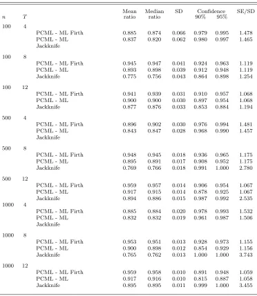
Table 2 reports the simulation results where we compare the finite sample performance of the proposed APE estimator (PCML - ML Firth) with the estimator forν based on the PCML estimator of γ and the uncorrected ML estimator ˆηi(˜γ) (PCML - ML) and with Dhaene and Jochmans (2015)’s half-panel jackknife bias corrected estimator (Jackknife) illustrated in Section 3.2. 9 Again we report the mean and the median of the ratio ˜ν/ν,
the standard deviation of ˜ν, the interval coverage at the confidence level 90% and 95%, and the mean ratio between the estimator standard error and standard deviation.10
Table 2 reports the simulation results, from which it emerges that the proposed esti-mator exhibits a better finite sample performance than the half-panel jackknife estiesti-mator. Notice also that the jackknife estimator for the dynamic logit model cannot be computed for T < 6, as clarified in Section 3.2. Clearly the finite sample performance of the pro-posed estimator deteriorates with respect to that of CML - ML Firth, as per the effect of the PCML estimator, which is not consistent whenγ 6= 0. Still, it can be noticed that the bias reduces rather quickly asT grows, as an effect of the use of the corrected ˜ηi(˜γ) in the computation of ˜ν, and that the proposed estimator represents a substantial improvement upon the half-panel jackknife in scenarios where T = 8,12.
5
Empirical application
We apply our proposed formulation to the problem of estimating the labor supply of married women. The same empirical application is considered by Fern´andez-Val (2009) and Dhaene and Jochmans (2015). The sample is drawn from the Panel Study of Income Dynamics (PSID), that consists ofn = 1,908 married women between 19 and 59 years of age in 1980, followed for T = 7 time occasions, from 1979 to 1985. We specify a static logit model for the probability of being employed at time t, conditional on the number of children of a certain age in the family, namely the number of kids between 0 and 2 years old, between 3 and 5, and between 6 and 17, on the husband’s income, and on the woman’s age and age squared. We also specify a dynamic logit model, that is we include lagged participation in the set of model covariates.
9
In the Monte Carlo study by Dhaene and Jochmans (2015), the APE estimator is computed for the covariate xit, which is associated with δ = 0 in the current design. We instead investigate the finite
sample performance of the APE estimator for the effect of yi,t−1. 10
Table 2: Simulation results for ˜ν, dynamic logit model
Mean Median SD Confidence SE/SD
n T ratio ratio 90% 95%
100 4
PCML - ML Firth 0.885 0.874 0.066 0.979 0.995 1.478 PCML - ML 0.837 0.820 0.062 0.980 0.997 1.465 Jackknife
100 8
PCML - ML Firth 0.945 0.947 0.041 0.924 0.963 1.119 PCML - ML 0.893 0.898 0.039 0.912 0.948 1.119 Jackknife 0.775 0.756 0.043 0.864 0.898 1.254
100 12
PCML - ML Firth 0.941 0.939 0.031 0.910 0.957 1.068 PCML - ML 0.900 0.900 0.030 0.897 0.954 1.068 Jackknife 0.877 0.876 0.033 0.853 0.884 1.194
500 4
PCML - ML Firth 0.896 0.902 0.030 0.976 0.994 1.481 PCML - ML 0.843 0.847 0.028 0.968 0.990 1.457 Jackknife
500 8
PCML - ML Firth 0.948 0.945 0.018 0.936 0.965 1.175 PCML - ML 0.895 0.891 0.017 0.908 0.952 1.175 Jackknife 0.769 0.766 0.018 0.991 1.000 2.780
500 12
PCML - ML Firth 0.959 0.957 0.014 0.906 0.954 1.067 PCML - ML 0.917 0.915 0.014 0.878 0.925 1.067 Jackknife 0.894 0.886 0.015 0.987 0.992 2.535 1000 4
PCML - ML Firth 0.885 0.884 0.020 0.978 0.993 1.532 PCML - ML 0.832 0.832 0.019 0.961 0.987 1.506 Jackknife
1000 8
PCML - ML Firth 0.953 0.951 0.013 0.928 0.973 1.155 PCML - ML 0.900 0.898 0.012 0.854 0.929 1.156 Jackknife 0.765 0.762 0.013 1.000 1.000 3.743
1000 12
PCML - ML Firth 0.959 0.958 0.010 0.891 0.948 1.059 PCML - ML 0.917 0.916 0.010 0.815 0.887 1.058 Jackknife 0.895 0.895 0.011 0.999 1.000 3.455
Notes: 1000 replications. PCML-ML Firth denotes the proposed estimator; PCML-ML denotes the estimator of the APE based on the PCML estimate ofβ and the uncorrected estimated ofηi(˜γ); Jackknife
Table 3: Female labor force participation: static logit model
Model parametersβ Average partial effectsµ
CML Jackknife CML - ML Firth CML - ML Jackknife
# Children 0-2 -1.183∗∗∗ -1.172∗∗∗ -0.096∗∗∗ -0.089∗∗∗ -0.106∗∗∗
(0.100) (0.121) (0.019) (0.017) (0.015) # Children 3-5 -0.909∗∗∗ -0.931∗∗∗ -0.074∗∗∗ -0.069∗∗∗ -0.084∗∗∗
(0.111) (0.133) (0.021) (0.019) (0.016) # Children 6-17 -0.272∗∗∗ -0.271∗∗ -0.022 -0.020 -0.024∗∗∗
(0.097) (0.115) (0.018) (0.017) (0.006) Husband income -0.014∗∗∗ -0.011∗ -0.001 -0.001 -0.001
(0.005) (0.006) (0.001) (0.001) (0.001)
Age 1.646∗ 1.714 0.006 0.006 0.018
(0.918) (1.086) (0.040) (0.037) (0.044) Age squared -0.224∗ -0.211
(0.127) (0.150)
Notes: standard errors in square brackets. ∗∗∗ p-value<0.01,∗∗ p-value<0.05,∗p-value<0.10. CML
denotes the Conditional Maximum Likelihood estimator; Jackknife denotes Hahn and Newey (2004)’s jackknife bias corrected estimator; CML-ML Firth denotes the proposed estimator; CML-ML denotes the estimator of the APE based on the CML estimate of β and the uncorrected estimated of αi(˜β).
Source: PSID 1979-1985.
The estimation results for the static logit model are reported in Table 3. We report both the CML and Hahn and Newey (2004)’s panel jackknife estimates of the model parameters. Despite the coefficients estimated by CML are all statistically significant at least at the 10% level, when we look at the estimated APE the model covariates do not seem to exert a significant effect on the probability of being employed, with the exception of having children between 0 and 2 years old, which reduces the probability of being employed by 9.6 percentage points, and having children between 3 and 5 years old, which reduces the probability by 7.4. It is worth noticing that CML and jackknife parameter estimates are quite similar, even thoughT is only 7 and the sample is around 2000. There is instead a noticeable difference in the standard errors, that are larger for the jackknife. The estimates of the APE seem to be along the same lines, whether obtained by the proposed estimator, the uncorrected CML-ML or the panel jackknife.
Table 4: Female labor force participation: dynamic logit model
Model parametersθ Average partial effectsν
PCML Jackknife PCML - ML Firth PCML - ML Jackknife
# Children 0-2 -0.909∗∗∗ -1.083∗∗∗ -0.060∗∗∗ -0.056∗∗∗ -0.107
(0.099) (0.141) (0.017) (0.016) (0.252) # Children 3-5 -0.555∗∗∗ -0.713∗∗∗ -0.037∗∗ -0.034∗∗ -0.073
(0.102) (0.149) (0.017) (0.016) (0.187)
# Children 6-17 -0.173∗ -0.136 -0.011 -0.011 -0.020
(0.093) (0.136) (0.016) (0.015) (0.103)
Husband income -0.009∗∗ -0.006 -0.001 -0.001 -0.001
(0.004) (0.006) (0.001) (0.001) (0.088)
Age 1.509∗ -0.152 0.013 0.012 -0.022
(0.827) (1.269) (0.031) (0.029) (0.139)
Age squared -0.185∗ -0.154
(0.111) (0.172)
Lagged participation 1.713∗∗∗ 2.200∗∗∗ 0.134∗∗∗ 0.127∗∗∗ 0.127
(0.103) (0.082) (0.022) (0.021) (0.137)
Notes: standard errors in square brackets. ∗∗∗ p-value < 0.01, ∗∗ p-value < 0.05, ∗ p-value < 0.10.
PCML denotes the Pseudo Conditional Maximum Likelihood estimator; Jackknife denotes Dhaene and Jochmans (2015)’s half-panel jackknife bias corrected estimator; PCML-ML Firth denotes the proposed estimator; PCML-ML denotes the estimator of the APE based on the PCML estimate of θ and the uncorrected estimated ofηi(˜θ). Source: PSID 1979-1985.
is large, and that the estimated APE amounts to 12.7 percentage points, similar to that obtained with PCML - ML Firth.11
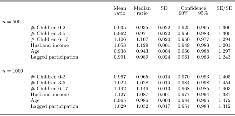
Our last exercise consists of a calibrated simulation study, in order to investigate the finite sample performance of the proposed estimator with a design close to a real data application.12 For the static and dynamic models, we draw n = 500,1000 women from
PSID, each observed for 7 time occasions, and estimate the model parameters obtaining ˜β
by CML for the static logit model and ˜θ by PCML for the dynamic logit model. We then use ˜β and ˜θ to generate data from a static or dynamic logit model, keeping the model covariates fixed and generating the error terms as a standard logistic random variables. We then re-estimate the model parameters and compute the APEs. The simulation is repplicated 1000 times.
The results for the static and dynamic logit models are reported in Tables 5 and 6, respectively. From Table 5 it emerges that the performance of the proposed estimator improves when n goes from 500 to 1000, and the results are comparable with those obtained with the simpler simulation design by Hahn and Newey (2004) in Section 4.1. Overall, the same happens for the dynamic logit as well, although in a less evident manner. Compared to the standard deviations, for both models standard errors are rather large,
11
The APE, however, is not statistically significant; Dhaene and Jochmans (2015) argue that this can be expected with half-panel jackknife, which may not be very precise with short T. They recommend using their half-panel jackknife correction of the objective function instead.
12
that however should be shrinking with larger T as suggested by the results in Section 4.
Table 5: Calibrated simulation results for the static logit model based on PSID 1979 -1985, CML-ML Firth
Mean Median SD Confidence SE/SD
ratio ratio 90% 95%
n= 500
# Children 0-2 0.917 0.917 0.019 0.804 0.892 1.212 # Children 3-5 0.941 0.941 0.018 0.916 0.956 1.233 # Children 6-17 1.220 1.208 0.017 0.749 0.863 1.225 Husband income 0.999 0.974 0.001 0.957 0.986 1.236
Age 0.853 0.877 0.003 0.973 0.989 1.322
n= 1000
# Children 0-2 0.977 0.975 0.015 0.926 0.971 1.167 # Children 3-5 0.999 1.001 0.015 0.935 0.976 1.128 # Children 6-17 1.143 1.144 0.012 0.825 0.913 1.179 Husband income 1.016 1.017 0.001 0.946 0.985 1.184
Age 1.014 1.010 0.003 0.951 0.983 1.187
Notes: 1000 replications. Source: PSID 1979 - 1985.
6
Concluding remarks
So far, the literature has proposed analytical or jackknife bias corrected APE estimators. They often depend on some bias corrected estimators of the slope coefficients, which are ensured to have confidence intervals centered at their probability limit only whenT grows faster than n1/3, meaning that they attain a good finite sample performance with rather
large T compared to n. This is rarely the case in microeconomic applications, where the number of subjects is often much larger than the number ot time occasions, especially in surveys with rotating sampling designs.
The method presented in this paper partly overcomes this issue by exploiting a fixed-T
consistent estimator of the slope coefficients of the logit model. The proposed estimator has asymptotic bias O(T−2
), but it is shown to perform well in finite samples, even when
n is much larger than T. Moreover, the bias corrected estimate of the unobserved het-erogeneity based on the modified score by Firth (1993) entails a substantial improvement over the standard ML estimate with short T.
Table 6: Calibrated simulation results for the dynamic logit model based on PSID 1979 - 1985, PCML-ML Firth
Mean Median SD Confidence SE/SD
ratio ratio 90% 95%
n= 500
# Children 0-2 0.935 0.935 0.022 0.925 0.965 1.306 # Children 3-5 0.962 0.971 0.022 0.956 0.983 1.300 # Children 6-17 1.106 1.107 0.020 0.950 0.977 1.294 Husband income 1.058 1.129 0.001 0.949 0.983 1.201
Age 0.938 0.943 0.004 0.966 0.988 1.297
Lagged participation 0.991 0.989 0.024 0.961 0.983 1.243
n= 1000
# Children 0-2 0.967 0.965 0.014 0.970 0.993 1.405 # Children 3-5 1.022 1.028 0.014 0.984 0.998 1.454 # Children 6-17 1.142 1.146 0.013 0.968 0.985 1.403 Husband income 1.127 1.087 0.001 0.977 0.994 1.387
Age 0.965 0.986 0.003 0.984 0.995 1.472
Lagged participation 1.029 1.032 0.017 0.954 0.983 1.312
Notes: 1000 replications. Source: PSID 1979 - 1985.
References
Andersen, E. B. (1970). Asymptotic properties of conditional maximum-likelihood esti-mators. Journal of the Royal Statistical Society, Series B, 32:283–301.
Barndorff-Nielsen, O. (1978). Information and Exponential Families in Statistical Theory. John Wiley & Sons.
Bartolucci, F. and Nigro, V. (2010). A dynamic model for binary panel data with unob-served heterogeneity admitting a √n-consistent conditional estimator. Econometrica, 78:719–733.
Bartolucci, F. and Nigro, V. (2012). Pseudo conditional maximum likelihood estimation of the dynamic logit model for binary panel data. Journal of Econometrics, 170(1):102– 116.
Chamberlain, G. (1980). Analysis of covariance with qualitative data. The Review of Economic Studies, 47:225–238.
Chamberlain, G. (1985). Heterogeneity, omitted variable bias, and duration dependence. In Heckman, J. J. and Singer, B., editors, Longitudinal analysis of labor market data. Cambridge University Press: Cambridge.
Chernozhukov, V., Fern´andez-Val, I., Hahn, J., and Newey, W. (2013). Average and quantile effects in nonseparable panel models. Econometrica, 81(2):535–580.
Cox, D. (1972). The analysis of multivariate binary data. Applied Statistics, 21:113–120.
Dhaene, G. and Jochmans, K. (2015). Split-panel jackknife estimation of fixed-effect models. The Review of Economic Studies, 82(3):991–1030.
Fern´andez-Val, I. (2009). Fixed effects estimation of structural parameters and marginal effects in panel probit models. Journal of Econometrics, 150(1):71–85.
Firth, D. (1993). Bias reduction of maximum likelihood estimates. Biometrika, 80(1):27– 38.
Hahn, J. and Kuersteiner, G. (2011). Bias reduction for dynamic nonlinear panel models with fixed effects. Econometric Theory, 27(6):1152–1191.
Hahn, J. and Newey, W. (2004). Jackknife and analytical bias reduction for nonlinear panel models. Econometrica, 72(4):1295–1319.
Hansen, L. P. (1982). Large sample properties of generalized method of moments estima-tors. Econometrica, 50:1029–1054.
Honor´e, B. E. and Kyriazidou, E. (2000). Panel data discrete choice models with lagged dependent variables. Econometrica, 68:839–874.
Hsiao, C. (2005). Analysis of Panel Data (2nd edition). Cambridge University Press, New York.
Lancaster, T. (2000). The incidental parameter problem since 1948. Journal of Econo-metrics, 95:391–413.
Neyman, J. and Scott, E. L. (1948). Consistent estimates based on partially consistent observations. Econometrica, 16:1–32.