Demand adjusted capital input and
potential output in the context of U.S.
economic growth
Bitros, George C.
Athens University of Economics and Business, Department of
Economics
25 May 2019
Demand adjusted capital input and potential output in the context of U.S. economic growth
George C. Bitros
Professor of Political Economy, Emeritus Athens University of Economics and Business 80 Patision Street, 6th Floor, Athens 104 34, Greece
Tel: +30 210 8203740 Fax: +30 210 8203301, E-mail: bitros@aueb.gr
Abstract
Two alternative measures of demand adjusted capital input for the U.S. non-farm private business sector are derived and their differential impacts on the potential supply of output are compared to those obtained using the unadjusted index of capital input published by the Congressional Budget Office (CBO). The re-sults show that, allowing for the demand pressure on the fixed assets of firms, leads to three effects. It
raises the level of estimated potential output well above CBO’s estimates; with the exception of the 1990s,
the estimated growth rates turn out to be higher than those computed by CBO; and, lastly, the long term trend of the growth rates with and without the demand adjustment to the capital input is sloping down-wards. The latter finding was not unexpected since aggregate demand, as reflected in the utilization rate of fixed assets by firms, has been trending downwards throughout the postwar period. Drawing on these find-ings it is concluded that the path to secular stagnation that the U.S. economy is following in the postwar period is not due solely to headwinds on the supply side. To some degree, perhaps significant, the deceler-ation in the expansion of productive capacity as well as in the intensity of its utilizdeceler-ation is due to the de-clining long term aggregate demand.
JEL Classification: E01, E22, O47
Keywords: Potential output, capital input, capital stock, economic growth, economic growth headwinds, secular stagnation
1. Introduction
The term output, with or without further qualification, is used to connote different things. For an example, consider the expression potential output. A cursory search in the relevant literature re-veals that some use it to imply the highest level of Gross Domestic Product (GDP) that can be pro-duced with a given mix of available resources and institutions; some others to signify the highest level of GDP that can be sustained over the long term; and still some others to denote the GDP that can be produced by an economy if all its resources are fully employed. This paper employs the fol-lowing three definitions. The first of them is employed by the Congressional Budget Office (2001,
1) to estimate past and future growth rates of “maximum sustainable GDP consistent with a stable rate of inflation”. In particular, as they explain in pages 8-9 of this publication, the approach by which they pursue this task is based on the Cobb-Douglas production function:
1 1
t t t t
Q A LK , (1) Potential output—the trend growth in the productive capacity of the economy—
is an estimate of the level of real GDP attainable when the economy is operating at a high rate of resource use. It is not a technical ceiling on output that cannot be exceeded. Rather, it is a measure of maximum sustainable output—the level of real GDP in a given year that is consistent with a stable rate of inflation.
Output supply is the value of goods and services produced within a certain period, say a quarter or a year. It corresponds to the real GDP reported in the National In-come and Product Accounts (NIPA).If output supply rises above potential output, constraints on productive capacity begin to bind, inflationary pressures build, and firms react by raising the utilization of their fixed assets. On the contrary, if output supply falls below potential output, resources are lying idle, inflationary pressures abate, and firms react by reducing the utilization of their fixed assets.
where the symbols are defined as follows: Qt= real GDP in year t; Lt = billion hours worked in
year t; Kt1= real value of the capital stock in year t-1; At = Total Factor Productivity (TFP) in year t; and the parameter
stands for the income share of capital in the value of output.Transforming (1) into logarithmic form, differentiating totally the resulting expression, and
setting
0.3 on account of the evidence that the payments to owners of capital have averaged roughly 30 percent of total U.S. income since 1947, yields:1
0 7 0 3
t t t t
% Q % A . % L . % K . (2) This equation states that the growth rate of GDP equals the growth rate of TFP plus the weighted average of the growth rates of labor and capital; Or, to express it in a way indicating that TFP is
computed as a residual, the growth rate of At is equal to the growth rate of Qt not accounted for by the weighted average of the growth rates ofLt and Kt.
Equation (2) holds generally. That is, it holds for any period, any value of , and any dis-aggregation, definition and measurement of the variables involved. Thus, by redefining it as:
1
%Qtp %Atp 0.7 % Ltp0.3 % Ktp , (3)
where the upper index pdenotes the “potential” values of the variables, the researchers of the Congressional Budget Office (henceforth CBO) proceed in two steps. In the first step, using (2) in conjunction with data from the U.S. Bureau of Economic Analysis (BEA), for the variables
and
t t
Q K , and the Bureau of Labor Statistics (BLS), for the variable Lt, they compute the growth rates of At going back to 1949. Past values vary due to both regular and irregular factors.
Therefore, to obtain the growth rates %Ltp and %Atp, the variables Lt and At are purged from
their cyclical components by taking their centered five year moving average. As for the growth
rate %Ktp, they obtain it by setting Kt1 Ktp1 on account of the rationalization that:
Lastly, upon inserting % , % and % 1
p p p
t t t
A L K
into (3), they obtain the trend growth rate
% p t
Q
as a weighted sum of the trend growth rates of labor and capital services plus the trend
growth rate in TFP.
Table A1 in the Appendix1 presents the time series of real GDP as a measure of output (Qt), the
labor (Lt) and capital (Kt1) inputs, and labor productivity (Qt /Lt). These constitute the series
re-ported in the sources mentioned at the bottom of the table. Table A2 reports the most recent
esti-mates and projections by CBO of potential output (Qtp) and its determinants. In the latter table the rows 1949-2016 refer to the historical estimates, whereas the rows 2017-2027 exhibit those that are
projected. Finally, in line with the preceding remark, according to which they set 1 1
p t t
K K , the
se-ries of capital input reported by CBO is the same in both tables.
In Bitros (2019a) the above analytical framework was adapted and applied in conjunction with data for the U.S. nonfarm private business sector to investigate the linkages between capital input and potential output over the period 1949-2016. More specifically, by focusing on the changes in
the composition of the capital stock in terms of structures, equipment and intangibles, average service lives, and relative prices of producer’s to consumer’s goods, that paper allowed for their influence on the capital input and traced the latter’s effects on potential output. From the results it emerged that when the capital input is revised to reflect all these changes in the capital stock, the potential supply of output decelerates even faster than suggested by CBO’s estimates and as a result the real economy in the years following the 2007 financial crisis appears to have adjusted to its lower potential faster than the protagonists of the secular stagnation hypothesis have sug-gested. But in as much as the deceleration of potential output is an undesirable development, it may not be due exclusively to the supply side headwinds discussed in that paper, since it may have trended downwards due also to slowing aggregate demand.
Thus, the focus in the present paper is to highlight the possible linkages of potential output sup-ply to influences that may emanate from the demand side of the economy. To this effect, Section 2 lays out the model which is employed in the empirical part. This task is accomplished by expanding along the lines pursued in Bitros (2019a). In particular, the adjustments in the capital input adopted there are taken a step further to allow for the changes in the intensity of the utilization of fixed
1
sets, drawing on the conceptualization that they associate closely with the changes in aggregate output demand. Section 3 comments on the proxy variable used to capture the effects of changes in aggregate demand that are channeled to the potential supply of output through the capital input. Given that the main body of the data used in the calculations coincides with those presented in the aforementioned study, the emphasis in this section is placed mainly on the issues regarding the def-inition, measurement and data sources of the utilization rate. Section 4 reports on the results and their possible significance and policy implications; and lastly, Section 5 closes with a summary of the main findings and conclusions.
2. Linking potential supply and demand for output
Let us go back to equation (2) and redefine it so as to explain the percentage growth rate of out-put supply in the light of the adjustments made to the capital inout-put in Bitros (2019a):
1
0 7 0 3
t t t ˆt
% Q % A . % L . % K . (4)
From the definition it follows that the left side of (4) stands for the percentage growth rate of real GDP produced and supplied in any given period. As for the right side, this shows the contribu-tions from three sources. Namely, the labor input, which corresponds to the percentage rate of change in the hours worked by workers, times 0.7; TFP, which is reckoned as a residual; and the percentage rate of change in the supply of the capital input times 0.3. The new element is the
cap-ital input, labeledKˆt1, which signifies that the capital stock has been adjusted for changes in: (a) its composition in terms of structures, equipment and intangibles, (b) the average service lives of these producer’s goods, and (c) their prices relative to consumer’s goods.
In view of its treatment by CBO, the quantity of capital services used may or may not coincide
with their available supply. The term % Kˆt1 in (4) stands for the percentage rate of change in the maximum available supply of the capital input. It is an upper limit that cannot be exceeded. But how much of it is utilized in the production process period in-period out depends on the de-mand for output. Therefore, to obtain an approximate measure of the capital input used by firms,
a convenient approach is to introduce the utilization rate (ut) of fixed assets, which measures the percentage of available productive capacity utilized at time t. More specifically, we propose to set
1 1 1
t t ˆt
aggregate output demanded. Thus, on account of this conceptualization, we may redefine (4) as in (5) below:
1
0 7 0 3
t t t t
% Q % A . % L . % K . (5)
Observe that in this specification we have changed the symbolAttoAt. We have done so to indicate that the percentage rate of change of TFP corresponds to the revised definition and measurement of capital
services. Finally, expressing (5) in terms of the potential values of the variables yields:
1
0 7 0 3
p p p p
t t t t
% Q % A . % L . % K . (6)
Now the differences between (3) and (6) are quite fundamental both from a theoretical and an empirical standpoint. Adopting the view that the available quantity of capital services represents their potential contribution to output, in essence CBO’s researchers maintain that the rate of po-tential economic growth is unrelated to capacity utilization. More specifically, even though they do not state it explicitly, they reason that while in the short run capacity utilization may affect the rate of economic growth due to price and other rigidities, in the long run the adjustments that take place in the economy render its influence irrelevant. Yet, numerous macroeconomic theorists have argued that the intensity with which firms use their fixed assets is too important to be ig-nored in the study of economic growth on at least three grounds. The first, emanating from a lengthy literature that includes contributions for example by Calvo (1975), Hulten (1986), Wen (1998) and Chatterjee (2005), establishes that capacity utilization relates positively to economic growth through the productivity channel. To see this linkage, assume that because of conditions that are inherent in production technologies, up to a point increases in capacity utilization raise productivity, whereas further increases thereafter lead to production bottlenecks and productivity declines. Under these circumstances the marginal cost of capacity utilization in terms of produc-tive efficiency would not be zero and firms might have good economic reasons to use their fixed
Unlike the productivity channel, which works through the supply side, the second ground for taking into account the linkage between capacity utilization and economic growth stems from a strand of literature that places sole emphasis on the demand side of the economy. Keynes (1936) was the first to point towards this direction. But his interest was in the study of the short run im-plications of aggregate demand and it was left to Harrod (1939), Khan (1959), Robinson (1962) and Kalecki (1971) to develop insightful dynamic models of the long run. Central to them all, as well as to the models presented more recently by researchers working in the their tradition, like for example Dutt (2006), Dutt, Ross (2007) and Shaikh (2009), is the role of capacity utilization as a channel of the influences from changes in aggregate demand to economic growth. Just to sketch the mechanism they envision to be at work, assume that we observe a very simple Keynes-Kalecki economy with the following characteristics:
Each unit of capital stockKtis operated by one unit of laborLt;
The capital stock is operated with intensityu, and hence the quantity of output
pro-duced Yt is equal touKt;
The total output is distributed in the form of wages wLtand profitsrKt, wherew and r
stand for the wage rate and the profit rate, respectively;2
While workers consume all of their income, profit earners save some proportions;
Profit earners invest their savings so that St srKt is always equal to investmentIt.
Now in this economy let the central bank reduce the discount rate to stimulate economic activity and combat unemployment. How might this policy influence economic growth and what might be the role in this regard of the utilization rateu?
The reduction in the discount rate would certainly encourage some firms to bring forward their investment plans. As a result, investment would be expected to accelerate. Assume that the new
higher level of planned investment is It* and that the new higher level of the capital stock
con-sistent with this investment isK*t . In turn, with u given, the planned supply of output will rise to
a new higher level, say * t
Y , and the same will happen to profits. Over time the share of profits will
increase enough so that the savings by profit earners will come to rest at the higher planned level
2It should be noted that the term “profits” corresponds to “
of investment where we will haveSt* I*t . From this analysis it follows that the reduction in the central bank discount rate motivates stimulation of aggregate demand by raising the level of planned investment and boosting economic growth. By how much it depends on the utilization rate
u, which in this case is held constant. However, having demonstrated the mechanism through which it works, it should not come as a surprise that according to this key model “demand creates its own supply”, i.e. the opposite of Say’s Law on which CBO’s approach is based.
Could thinking along these lines offer some clues to the situation that emerged in the U.S. af-ter the 2009 financial crisis? For this particular period CBO revised downwards its estimates of potential output by 5% due largely to reduced labor and capital inputs. But the Federal Reserve authorities could not do much because the policy interest rate had been reduced already closed to zero, so investment could not be stimulated through this channel. As a result many wandered:
Could the reduction in the capital and labor inputs be due to the lack of demand and not of sup-ply? Some world renowned economists thought that this might be the case and suggested policy initiatives to stimulate aggregate demand. For an example, consider Summers (2014a). Having returned to this question again and again since Summers (2013), in page 71 of this paper he an-swers by stating:
We are seeing very powerfully a kind of inverse Say’s Law. Say’s Law was the proposition that supply creates its own demand. Here, we are observing that lack of demand creates its own lack of supply.
and in page 72 he goes on to recommend, among several other policies, that:
The preferable strategy, I would argue, is to raise the level of demand at any giv-en rate of interest—raising the level of output consistent with an increased level of equilibrium rates and mitigating the various risks associated with low interest rates that I have described.
Yet, perhaps because at the time the U.S. Economy was on its way back to meaningful rates of economic growth, shortly thereafter Summers (2014b) moved away from his emphasis on the
lack of aggregate demand and in the direction of researchers who stress the lack of supply by ex-panding on Gordon’s (2014) headwinds that forestall it.
be given proper weight. The relevant literature is not void in this quest; Slowly and rather quietly research in this direction has made considerable progress. Although these efforts started some-what earlier than the breakout of the financial crisis in 2009, three notable contributions since then are the ones by Dutt (2010), Ferri et al (2011) and Fazzari et al. (2013). If one has to single out only one common element in the models they present, this is none other than capacity utiliza-tion. That is why they provide even stronger support than the two grounds we invoked above to justify the introduction into (3) aggregate demand considerations through this channel.
To conclude this summary into the theoretical and empirical reasons that warrant the applica-tion of (3) in the form of (6), we find it least creative to take sides as to whether in any period and under any circumstances Say’s Law holds sway directly or inversely. In our view in market economies with private ownership of the means of production economic growth is spearheaded other times by supply and other times by demand. So adopting a framework of analysis in which both are allowed to drive the course of potential output is prudent and may prove highly reward-ing in terms of explanatory power.
3. Capacity utilization and potential capital input
Regarding the utilization of productive capacity in the U.S, the database maintained by the Fed-eral Reserve Bank of St’ Louis provides time series at various sectoral levels. The one most rele-vant to this research is the index labelled “total capacity utilization”. But this index goes back on-ly to 1966 and, in as much as we searched for alternative sources of information that might
ena-ble us to extend it backwards to match the CBO historical statistics, i.e. to 1949, it proved impos-sible. For this reason, we adopted the following procedure. The same database reports an index labelled “manufacturing capacity utilization” which goes back to 1947. Thus, assuming that total economic activity correlates strongly with the activity in the manufacturing sector, we regressed the
index of total economy capacity utilization (tcut) on the index of manufacturing capacity utiliza-tion (mcut) and obtained the following equation:3
2
12 295 0 862 (9 73) (53.9)
0 981 (1,49)=2903.9, ( )=0.0000
t t
tcu . . mcu
.
R . , F P F
(7)
3
With its help we then extended the index tcutback to 1949. These series are displayed in Figure 1. Observe that over the period 1966-2016 the index mcuttracks tcutexceedingly well. By impli-cation, the strong fit of equation (7) ascertains that using it to project the series of total economy capacity utilization back to 1949 should not involve significant errors of measurement. How suc-cessfully this procedure performs is corroborated by the tight tracking of the solid line by the dot-ted extension of the dashed line.
Looking closer at this figure several significant observations come to mind. One, and perhaps most striking, is that with the exception of 1952 and 1965, which were war years for the U.S., the capacity utilization since 1949 never exceeded 87%. Actually, excluding the years of the Korean
the two lowest historical values in the abridged series of capital utilization, draw a straight line through them, construct an index of relative demand pressure by drawing on the deviations of total capacity utilization from the calculated straight line, and lastly, use this index of demand pressure to compute a demand adjusted series of the capital input.
A second observation is that the time trend of capacity utilization is negative. Why is this so? From Bitros (2019a) we know that the composition of the capital stock has been changing all these decades in favor of equipment and intangibles and against infrastructures. Could this shift have anything to do with the long term decline in the capacity utilization? Infrastructural invest-ments are generally more discrete and experience higher degrees of duplication than machinery and software. So the decline in their share in the capital stock would be expected to increase, not reduce capacity utilization. And the same is true with the advancement in automation which tends to favor relatively more the equipment part of the capital stock rather than that of infrastructure. Hence, even though we could not find hard evidence in this regard, most a priori considerations indicate that the culprit in the long term decline of capacity utilization may be associated with the decline in aggregate demand. Moreover, given that during the same period productive capacity as indexed by the ratio of net investment to the capital stock trended downwards at least in manufac-turing,4 the likelihood that both productive capacity and its utilization trended downwards mainly because of slackening aggregate demand does not seem baseless. But then capacity utilization influences potential capital input systematically and hence it should be treated as such by placing
emphasis on the demand adjusted series of potential capital input.
Lastly, notice that capacity utilization traces two cycles. One that moves upwards from the middle of the 1950s and ends in a trough around 1980 and another that turns again upwards around the 1980s, reaches an apex in the middle of the 1990s, and since then it has been declin-ing. These cycles are very lengthy and don’t have much in common with the forces that drive the normal business cycles in the U.S. economy. Rather they are associated with protracted swings in production technologies and shifting consumer tastes, income distribution and economic policies. By implication, failing to account for the effects of relative demand pressure, channeled to poten-tial capital input through capacity utilization, may introduce systematic biases into the estimates of potential output. To highlight this possibility, we carried out two separate calculations of the
4
mand adjusted potential capital input: One based on CBO’s capital input index Kt1and another based of the capital input Kˆt1 derived in Bitros (2019a). Both these series are shown in Columns (1)
and (2) of Table A4. In turn, the series Kt1 and Kˆt1 were multiplied by the index of relative
de-mand pressure rdpt shown in Column (3), and their five year centered moving average series are
report-ed under the symbols Kt1 and Kt1 in Columns (4) and (5), respectively.
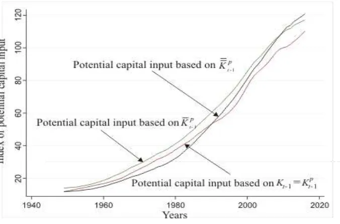
Figure 2 displays the graphs of the seriesK t1KtP1,Ktp1 and Ktp1. Observe that the graph of
1
p t
K lies above that ofKtp1 throughout the period under consideration, whereas the graph of 1
p t
K
crosses the latter from below beginning in the 1990s. Therefore, by ignoring the influences of aggre-gate demand that are channeled to aggreaggre-gate supply through the utilization rate, the deceleration
in recent years of potential output, and hence of economic growth, may have been less ominous than perceived by supply-siders. The objective of the presentation in the next section is to shed some light on this particular issue.
4. Potential output under alternative demand adjusted measures of capital input
[image:13.612.154.492.321.544.2]Table A5. As indicated earlier, CBO researchers have computed the series of potential output
us-ing in equation (3) the convention that 1 1
p t t
K K . However, above we argued in support of the
indices Kt1 and Kt1 to account for the influences of aggregate demand via the channel of the utili-zation rate. Therefore the remaining task is to compute equation (6) under the alternative demand adjusted measures of potential capital input and assess the differences. Notice that in (7a) below we
have changed the symbol % p t
Q
to% p t
Q
. We have done so for two reasons: First, to indicate that
applying this equation to the data reported by CBO does not give exactly their figures for potential out-put; and secondly, to hold the method of computation the same across all three equations.
1
1
1
0 7 0 3 (a)
0 7 0 3 (b)
0 7 0 3 (c)
p p p p
t t t t
p p p p
t t t t
p p p p
t t t t
% Q % A . % L . % K
% Q % A . % L . % K
% Q % A . % L . % K
(7)
Columns (3), (4) and (5) of Table A5 show the series of potential output computed by applying (7) to
the data. The series for potential output under the labels p and p t t
Q Q are much closed together. So, for
these two series together with that of actual outputQt. Observe that throughout the period under consider-ation the graph of the demand adjusted potential supply of output (Qtp ) lies above that computed in the absence of such adjustment (Qtp). What this finding implies is that above normal demand pressure on the fixed assets of firms shifts the potential supply of output upwards by leading to more intensive usage of
the available capital stock as well as stirring up additional new investment. Or, stating the same inference
in another way, gauging aggregate output supply in isolation from aggregate output demand results in an
underestimation of potential output because in line with Summers’s intuition the “lack of demand creates
its own lack of supply”.
However, aside from their differences in the levels, observe that the curves p and p t t
Q Q in
Fig-ure 3 differ also, albeit not widely, in their curvatFig-ures. The latter reflect the possible differences in the growth rates of the potential output from the two estimates. Thus, to highlight them we computed and in Figure 4 we present the 10 year average growth rates from the two series.
From them it turns out that with the exception of the period in the 1990s, allowing for the de-mand pressure on the fixed assets of firms in the postwar period would have resulted in higher growth rates of the potential supply of output relative to those estimated by CBO. But otherwise one cannot fail to observe that by both estimates their downward long term trend remains intact. This transpires because, even though allowing for the impact of aggregate demand would lead to
not been sufficiently robust to reverse their downward trend. Rather on the contrary, as docu-mented by the long term decline in the utilization rate, aggregate demand has been trending downwards throughout these decades because of its own strong headwinds. By all indications then the U.S. economy has entered into a prolonged period of secular stagnation due to economic growth retardants that operate through both aggregate supply and aggregate demand. For this rea-son, in addition to the supply side headwinds, it is high time to identify and confront the forces that are reliable for the long term decline in aggregate demand.
5. Summary of findings and conclusion
CBO researchers estimate potential output by relying on the traditional Solow type growth ac-counting approach. When they reckon the flow of capital services, they postulate that the poten-tial use of such services is equal to their available supply, because “the potential flow of capital ser-vices will always be related to the total size of the capital stock, not to the amount currently being used.”
However, be this as it may, there is considerable literature establishing that the potential flow of capital
services is not related to the total size of the capital stock but to that which is useable on rational
entrepre-neurial grounds. The introduction in the estimations of potential output of demand-side considerations via
the utilization rate is based on this conceptualization.
In particular, we derived two alternative measures of demand adjusted capital input for the U.S.
non-farm private business sector and compared their differential impacts on the potential supply of output
rela-tive to the unadjusted index of capital input published by CBO. The results from these comparisons
showed that, allowing for the demand pressure on the fixed assets of firms, leads to three effects. It raises
the levels of estimated potential output well above CBO’s estimates; with the exception of the 1990s, the
estimated growth rates turn out to be higher than those computed by CBO; and, lastly, the long term trend
of the growth rates with and without the demand adjustment of the capital input is sloping downwards.
The latter finding was not unexpected because aggregate demand as reflected in the utilization rate of
fixed assets by firms has been trending downwards throughout the postwar period.
Drawing on these findings we conclude that the path to secular stagnation that the U.S. economy is
fol-lowing in the postwar period is not due solely to headwinds on the supply side. The deceleration in the
expansion of productive capacity as well as in the intensity of its utilization cannot be explained in
Isola-tion to the trends that prevail in the aggregate demand. So it is high time that research economists turn
6. References
Bitros, G. C., (2019a), “Potential output, capital input and U.S. economic growth,”
https://www.dept.aueb.gr/sites/default/files/econ/dokimia/wp-03-2019-Bitros-200419.pdf .
Calvo, G., (1975), “Efficient and optimal utilization of capital services,” American Economic Re-view, 65, 181–186.
Chatterjee, S., (2005), “Capital utilization, economic growth and convergence,” Journal of Eco-nomic Dynamics & Control, 29, 2093–2124.
Dutt, A. K., (2006), “Aggregate Demand, Aggregate Supply and Economic Growth,” Interna-tional Review of Applied Economics, 20, 319–336.
Dutt, A. K., (2010), “Reconciling the growth of aggregate demand and aggregate supply,” in M. Setterfield (ed.), Handbook of Alternative Theories of Economic Growth, Northampton, MA: Edward Elgar, 220–240.
Dutt, A. K., Ross, J., (2007), “Aggregate demand shocks and economic growth,” Structural Change and Economic Dynamics, 18, 75–99.
Fazzari, S. M., Ferri, P. E., Greenberg, E. G., Variato, A. M., (2013), “Aggregate demand, instability, and growth,” Review of Keynesian Economics, 1, 1–21.
Ferri, P., Fazzari, S. M., Greenberg, E., Variato, A. M., (2011), “Aggregate demand, Harrod’s instability and fluctuations,” Computational Economics, 38, 209–220.
Gordon, R. J., (2014), “US Economic Growth is Over: The Short Run meets the Long Run,” in THINK
TANK 20: Growth, Convergence and Income Distribution: The Road from the
Bris-bane G-20 Summit, https://www.brookings.edu/.../2016/07/tt20-united-states
-economic-growth-gordon.pdf .
---, (2015), Beyond the Rainbow: The Rise and Fall of Growth in the American Standard of
Living, Princeton, NJ: Princeton University Press.
Harrod, R.F., (1939), “An essay in dynamic theory,” Economic Journal, 49, 14–33.
Hulten, C. R., (1986), “Productivity Change, Capacity Utilization, and the Sources of Efficiency Growth,” Journal of Econometrics, 33, 31–50.
Kahn, R. F., (1959). "Exercises in the analysis of growth," Oxford Economic Papers, 11, 143-56.
Kalecki, M., (1971), Selected Essays on the Dynamics of the Capitalist Economy, Cambridge,
Keynes, J. M., (1936), The General Theory of Employment, Interest, and Money, Cambridge, UK: Cambridge University Press.
Robinson, J., (1962). Essays in the Theory of Economic Growth, London: Macmillan.
Schultze, C. L., (1963), “Uses of Capacity Measures for Short-Run Economic Analysis,” Ameri-can Economic Review, Papers and Proceedings, 53, 293–308.
Shaikh, A., (2009), “Economic policy in a growth context: a classical synthesis of Keynes and Harrod,” Metroeconomica, 60, 455–494.
Skott, P., Zipperer, B., (2012), “An empirical evaluation of three post-Keynesian models,” Inter-vention: European Journal of Economics and Economic Policies, 9, 277–308. Summers, L. H., (2013), “IMF Fourteen Annual Research in Honor of Stanley Fisher,” in
Http://larrysummers.com/imf-fourteen-annual-research-in-honor-of-stanley-fisher/.
Summers, L. H., (2014), “U.S. Economic Prospects: Secular Stagnation, Hysteresis, and the Zero Lower Bound,” Business Economics, 49, 65-73.
APPENDIX
Table A1: Actual data underlying CBO’s computations of potential GDP
in the U.S nonfarm private business sector
Year GDPQt
(1) t L (2) 1 t K (3) Labor productivity (4)=(1):(2)
Year GDPQt
(1) t L (2) 1 t K (3) Labor productivity (4)=(1):(2) 1949 1950 1951 1952 1953 1954 1955 1956 1957 1958 1959 1960 1961 1962 1963 1964 1965 1966 1967 1968 1969 1970 1971 1972 1973 1974 1975 1976 1977 1978 1979 1980 1981 1982 1983 1984 1985 1,309 1,441 1,548 1,595 1,675 1,650 1,790 1,823 1,860 1,823 1,975 2,010 2,053 2,194 2,295 2,448 2,624 2,812 2,865 3,018 3,110 3,105 3,222 3,438 3,687 3,631 3,571 3,826 4,044 4,312 4,455 4,415 4,517 4,373 4,657 5,047 5,262 83.4 80.1 82.7 86.6 87.5 89.7 86.7 90.1 92.4 91.8 88.0 92.0 92.6 91.6 93.6 94.6 98.7 103.0 103.7 106.0 109.3 107.9 107.3 111.3 115.9 116.2 111.4 115.6 120.0 126.0 130.3 129.5 130.9 128.1 130.3 138.1 142.0 11.8 12.1 12.6 13.0 13.5 13.9 14.3 14.8 15.3 15.8 16.2 16.7 17.2 17.9 18.5 19.2 20.0 21.1 22.3 23.4 24.5 25.6 26.7 27.7 29.0 30.4 31.6 32.4 33.3 34.5 35.9 37.4 38.9 40.3 41.6 42.9 44.8 15.7 16.2 16.8 17.4 17.9 18.2 18.5 18.8 19.3 19.8 20.3 20.8 21.4 22.0 22.6 23.2 23.9 24.8 25.7 26.5 27.3 28.0 28.5 28.9 29.4 29.9 30.4 30.8 31.2 31.7 32.2 32.3 32.3 32.7 33.2 33.7 34.4 1986 1987 1988 1989 1990 1991 1992 1993 1994 1995 1996 1997 1998 1999 2000 2001 2002 2003 2004 2005 2006 2007 2008 2009 2010 2011 2012 2013 2014 2015 2016 5,463 5,658 5,916 6,134 6,228 6,191 6,442 6,642 6,950 7,191 7,516 7,909 8,325 8,789 9,173 9,240 9,404 9,697 10,131 10,513 10,848 11,097 10,954 10,488 10,823 11,061 11,406 11,633 12,015 12,426 12,611 143.4 148.0 152.4 157.2 157.3 154.3 154.7 158.8 165.3 169.6 173.4 179.2 184.1 188.1 191.3 188.4 184.8 183.2 185.6 188.9 193.1 195.1 192.7 180.2 180.4 184.8 188.8 192.5 196.9 201.3 204.6 46.6 48.3 49.9 51.5 53.2 54.6 55.8 57.1 58.7 60.6 62.9 65.6 68.8 72.5 76.5 80.3 83.2 85.2 87.1 89.2 91.7 94.5 97.3 99.3 100.0 100.8 102.2 104.0 105.9 108.0 110.3 35.1 35.8 36.5 37.3 38.0 38.6 39.1 39.6 40.2 40.7 41.5 42.6 44.0 45.5 47.2 48.8 50.3 51.5 52.9 54.1 55.2 56.2 57.1 57.9 58.4 58.9 59.5 60.2 60.8 61.6 62.4 Notes
1. Actual GDP in billions of chained 2009 dollars.
2. Actual hours worked, billions of hours. Data from 1964 to 2016 from U. S. Bureau of Labor Statistics (BLS), Division of Major Sector Productivity, August 18, 2017. Data for 1949 to 1963, computed backwards using the percentages of annual change from BLS series PRS85006032.
3. Capital Services, index: 2009 = 100, lagged one year.
Table A2: Historical and projected potential values of GDP and its determinants in the U.S nonfarm private business sector
Year
P p t t
GDP Q
(1) P t L (2) 1 1 p t t K K
(3)
P t
A
(4) Year
P t GDP (1) P t L (2) 1 1 p t t K K
(3) P t A (4) 1949 1950 1951 1952 1953 1954 1955 1956 1957 1958 1959 1960 1961 1962 1963 1964 1965 1966 1967 1968 1969 1970 1971 1972 1973 1974 1975 1976 1977 1978 1979 1980 1981 1982 1983 1984 1985 1986 1987 1988 1,341 1,412 1,481 1,558 1,629 1,680 1,722 1,768 1,823 1,891 1,962 2,041 2,123 2,210 2,309 2,412 2,520 2,637 2,769 2,906 3,041 3,160 3,271 3,387 3,508 3,653 3,806 3,945 4,086 4,241 4,399 4,516 4,620 4,773 4,944 5,129 5,336 5,548 5,753 5,949 85.5 87.2 88.1 89.3 91.1 92.3 93.1 93.9 94.7 95.6 96.8 98.1 99.3 100.5 102.2 103.9 105.3 106.5 107.8 109.5 111.2 112.9 114.9 117.3 119.4 122.0 125.0 128.0 130.9 133.7 136.6 139.8 143.0 146.1 149.1 152.2 155.2 158.0 160.7 162.9 11.8 12.1 12.6 13.0 13.5 13.9 14.3 14.8 15.3 15.8 16.2 16.7 17.2 17.9 18.5 19.2 20.0 21.1 22.3 23.4 24.5 25.6 26.7 27.7 29.0 30.4 31.6 32.4 33.3 34.5 35.9 37.4 38.9 40.3 41.6 42.9 44.8 46.6 48.3 49.9 46.4 47.8 49.1 50.5 51.5 52.1 52.6 53.1 53.8 54.9 56.1 57.4 58.6 59.9 61.2 62.5 63.8 65.2 66.6 68.1 69.4 70.3 70.9 71.6 72.3 73.2 74.2 75.2 76.3 77.3 78.2 78.1 77.8 78.4 79.4 80.5 81.5 82.6 83.7 84.8 1989 1990 1991 1992 1993 1994 1995 1996 1997 1998 1999 2000 2001 2002 2003 2004 2005 2006 2007 2008 2009 2010 2011 2012 2013 2014 2015 2016 2017 2018 2019 2020 2021 2022 2023 2024 2025 2026 2027 6,142 6,332 6,508 6,680 6,869 7,080 7,313 7,564 7,871 8,242 8,639 9,035 9,415 9,737 10,015 10,290 10,569 10,809 11,016 11,226 11,405 11,525 11,657 11,829 12,033 12,257 12,492 12,719 12,943 13,191 13,459 13,740 14,033 14,339 14,655 14,977 15,306 15,642 15,986 164.7 166.5 168.4 170.7 173.4 176.3 179.6 182.4 184.9 187.4 189.7 191.3 192.8 193.8 194.3 194.7 195.2 195.7 196.0 196.5 197.1 197.4 197.9 198.8 200.0 201.4 202.9 203.9 204.6 205.4 206.2 207.0 207.8 208.6 209.5 210.4 211.3 212.2 213.0 51.5 53.2 54.6 55.8 57.1 58.7 60.6 62.9 65.6 68.8 72.5 76.5 80.3 83.2 85.2 87.1 89.2 91.7 94.5 97.3 99.3 100.0 100.8 102.2 104.0 105.9 108.0 110.3 112.6 115.0 117.7 120.4 123.0 125.6 128.3 130.9 133.7 136.5 139.4 85.9 86.9 87.8 88.7 89.5 90.4 91.3 92.3 93.9 95.8 97.9 100.0 102.0 103.9 105.9 107.9 109.8 111.1 111.9 112.7 113.5 114.3 115.1 115.9 116.7 117.5 118.3 119.2 120.1 121.1 122.3 123.5 124.9 126.3 127.8 129.3 130.9 132.4 134.0 Notes
1. Potential GDP in billions of chained 2009 dollars. 2. Potential hours worked in billions of hours.
3. Cyclically unadjusted capital Services, index: 2009 = 100, lagged one year. Hence, Kt1KtP1. 4. Potential Total Factor Productivity, index: 2000 = 100
Source: CBO's June 2017 report: An Update to the Budget and Economic Outlook: 2017 to 2027,
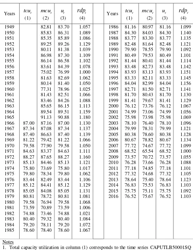
Table A3: Indices of capacity utilization and relative demand pressure
Years tcut
(1) t mcu (2) t u (3) t rdp
(4) Years
t tcu (1) t mcu (2) t u (3) t rdp (4) 1949 1950 1951 1952 1953 1954 1955 1956 1957 1958 1959 1960 1961 1962 1963 1964 1965 1966 1967 1968 1969 1970 1971 1972 1973 1974 1975 1976 1977 1978 1979 1980 1981 1982 1983 1984 1985 87.00 87.34 87.40 81.22 79.58 84.63 88.27 85.13 75.80 79.80 83.44 85.12 85.05 80.81 79.58 73.59 74.88 80.40 79.20 78.60 82.81 85.83 85.35 89.25 80.11 86.98 86.14 83.61 75.02 81.63 80.14 77.31 81.43 83.46 85.65 89.54 91.13 87.16 87.08 86.63 79.42 77.90 83.37 87.65 84.46 73.69 78.34 82.49 84.41 84.08 78.72 76.94 70.89 73.46 79.32 78.11 78.40 83.70 86.31 85.89 89.26 81.38 87.30 86.58 84.39 76.99 82.69 81.40 78.96 82.51 84.26 86.15 89.51 90.88 87.00 87.34 87.40 81.22 79.58 84.63 88.27 85.13 75.80 79.80 83.44 85.12 85.05 80.81 79.58 73.59 74.88 80.40 79.20 78.60 1.057 1.089 1.086 1.129 1.039 1.109 1.102 1.078 1.000 1.062 1.050 1.025 1.066 1.088 1.113 1.159 1.180 1.130 1.137 1.139 1.066 1.050 1.111 1.160 1.121 1.017 1.062 1.106 1.129 1.131 1.081 1.068 1.006 1.021 1.084 1.072 1.067 1986 1987 1988 1989 1990 1991 1992 1993 1994 1995 1996 1997 1998 1999 2000 2001 2002 2003 2004 2005 2006 2007 2008 2009 2010 2011 2012 2013 2014 2015 2016 81.16 84.30 83.77 82.48 79.90 80.49 81.44 83.48 83.93 83.33 84.04 82.71 81.70 81.41 76.12 74.99 75.98 78.10 79.99 80.38 80.67 77.72 68.52 73.57 76.28 77.18 77.32 78.64 76.83 75.75 76.52 80.97 84.03 83.30 81.64 78.55 79.53 80.41 82.73 83.13 82.11 82.99 81.50 80.43 79.67 73.76 73.06 73.98 76.40 78.31 78.60 78.82 74.67 65.54 70.72 73.66 74.85 74.68 75.40 75.53 75.11 75.67 81.16 84.30 83.77 82.48 79.90 80.49 81.44 83.48 83.93 83.33 84.04 82.71 81.70 81.41 76.12 74.99 75.98 78.10 79.99 80.38 80.67 77.72 68.52 73.57 76.28 77.18 77.32 78.64 76.83 75.75 76.52 1.099 1.140 1.135 1.121 1.092 1.101 1.114 1.142 1.151 1.145 1.156 1.141 1.130 1.129 1.067 1.056 1.069 1.096 1.121 1.128 1.134 1.099 1.000 1.055 1.088 1.101 1.105 1.123 1.103 1.092 1.103 Notes
1. Total capacity utilization in column (1) corresponds to the time series CAPUTLB50001SQ
from the database of the Federal Reserve Bank of St’ Louis.
2. Manufacturing capacity utilization in column (2) corresponds to the time series CA-PUTLB00004SQ from the database of the Federal Reserve Bank of St’ Louis.
Table A4: Alternative estimates of the demand adjusted potential capital input in the U.S nonfarm private business sector1
Years 1 1
p t t
K K
(1) 1 ˆt K (2) t rdp (3) 1 p t K (4) 1 p t K (5)
Years Kt1
(1) 1 ˆt K (2) t rdp (3) 1 p t K (4) 1 p t K (5) 1949 1950 1951 1952 1953 1954 1955 1956 1957 1958 1959 1960 1961 1962 1963 1964 1965 1966 1967 1968 1969 1970 1971 1972 1973 1974 1975 1976 1977 1978 1979 1980 1981 1982 1983 1984 1985 11.8 12.1 12.6 13.0 13.5 13.9 14.3 14.8 15.3 15.8 16.2 16.7 17.2 17.9 18.5 19.2 20.0 21.1 22.3 23.4 24.5 25.6 26.7 27.7 29.0 30.4 31.6 32.4 33.3 34.5 35.9 37.4 38.9 40.3 41.6 42.9 44.8 10.2 10.4 10.7 10.9 11.1 11.5 11.8 12.1 12.6 13.0 13.3 13.6 13.9 14.2 14.7 15.2 15.8 16.6 17.5 18.3 19.1 20.0 20.6 21.3 22.1 23.1 24.1 24.6 25.3 26.3 27.5 29.0 30.4 31.9 33.3 34.6 36.7 1.057 1.089 1.086 1.129 1.039 1.109 1.102 1.078 1.000 1.062 1.050 1.025 1.066 1.088 1.113 1.159 1.180 1.130 1.137 1.139 1.066 1.050 1.111 1.160 1.121 1.017 1.062 1.106 1.129 1.131 1.081 1.068 1.006 1.021 1.084 1.072 1.067 13.9 14.2 14.4 14.5 14.7 15.2 15.6 16.0 16.5 17.2 17.9 18.6 19.4 20.4 21.4 22.3 23.3 24.4 25.7 26.9 27.8 28.8 30.0 31.2 32.4 33.7 35.0 35.9 36.8 38.1 39.6 41.0 42.6 44.3 46.1 48.0 49.8 11.7 11.9 12.0 12.1 12.3 12.6 12.9 13.2 13.5 14.0 14.5 15.0 15.6 16.3 17.0 17.7 18.4 19.2 20.1 20.9 21.5 22.2 23.1 23.9 24.8 25.8 26.8 27.5 28.3 29.5 30.8 32.2 33.7 35.5 37.4 39.4 41.4 1986 1987 1988 1989 1990 1991 1992 1993 1994 1995 1996 1997 1998 1999 2000 2001 2002 2003 2004 2005 2006 2007 2008 2009 2010 2011 2012 2013 2014 2015 2016 46.6 48.3 49.9 51.5 53.2 54.6 55.8 57.1 58.7 60.6 62.9 65.6 68.8 72.5 76.5 80.3 83.2 85.2 87.1 89.2 91.7 94.5 97.3 99.3 100.0 100.8 102.2 104.0 105.9 108.0 110.3 38.9 40.9 42.7 44.5 46.6 48.5 49.9 51.5 53.3 55.5 58.1 61.0 64.3 68.0 72.2 76.5 79.7 81.7 83.6 86.0 89.1 92.6 96.4 99.5 100.0 101.4 103.5 106.2 109.0 112.3 115.6 1.099 1.140 1.135 1.121 1.092 1.101 1.114 1.142 1.151 1.145 1.156 1.141 1.130 1.129 1.067 1.056 1.069 1.096 1.121 1.128 1.134 1.099 1.000 1.055 1.088 1.101 1.105 1.123 1.103 1.092 1.103 51.9. 54.0 56.0 58.2 60.3 62.5 64.4 66.6 69.0 71.3 73.8 76.5 79.3 82.3 85.4 88.5 91.4 93.4 95.7 98.4 101.0 103.4 105.8 107.7 109.4 111.2 112.0 113.8 115.1 116.2 117.2 43.7 46.0 48.3 50.7 53.1 55.6 57.9 60.3 63.0 65.6 68.3 71.3 74.4 77.6 81.0 84.3 87.6 89.9 92.8 95.9 99.0 101.9 104.9 107.5 110.1 112.7 114.0 116.2 117.8 119.2 120.8 Notes
1. Capital input in column (1) as reported by CBO (see Table A1 and A2 above)
2. Capital input in column (2) from Bitros (2017). Computed to allow for compositional and other changes in the capital stock in the U.S nonfarm private business sector.
Table A5: Potential output under alternative demand adjusted estimates of potential capital input in the U.S nonfarm private business sector
Years Qt
(1) p t Q (2) p t Q (3) 1 p t Q (4) 1 p t Q (5)
Years Qt
(1) p t Q (2) p t Q (3) 1 p t Q (4) 1 p t Q (5) 1949 1950 1951 1952 1953 1954 1955 1956 1957 1958 1959 1960 1961 1962 1963 1964 1965 1966 1967 1968 1969 1970 1971 1972 1973 1974 1975 1976 1977 1978 1979 1980 1981 1982 1983 1984 1985 1,309 1,441 1,548 1,595 1,675 1,650 1,790 1,823 1,860 1,823 1,975 2,010 2,053 2,194 2,295 2,448 2,624 2,812 2,865 3,018 3,110 3,105 3,222 3,438 3,687 3,631 3,571 3,826 4,044 4,312 4,455 4,415 4,517 4,373 4,657 5,047 5,262 1,341 1,412 1,481 1,558 1,629 1,680 1,722 1,768 1,823 1,891 1,962 2,041 2,123 2,210 2,309 2,412 2,520 2,637 2,769 2,906 3,041 3,160 3,271 3,387 3,508 3,653 3,806 3,945 4,086 4,241 4,399 4,516 4,620 4,773 4,944 5,129 5,336 1,341 1,410 1,476 1,547 1,617 1,665 1,705 1,750 1,801 1,868 1,939 2,020 2,098 2,188 2,283 2,384 2,486 2,601 2,724 2,855 2,981 3,092 3,197 3,311 3,431 3,576 3,729 3,870 4,020 4,177 4,339 4,459 4,567 4,721 4,895 5,080 5,281 1,386 1,447 1,518 1,581 1,655 1,719 1,792 1,848 1,897 1,970 2,041 2,139 2,222 2,325 2,435 2,561 2,664 2,776 2,901 3,022 3,142 3,259 3,379 3,506 3,636 3,779 3,934 4,075 4,219 4,355 4,497 4,662 4,844 5,027 5,199 5,377 5,551 1,374 1,436 1,509 1,574 1,650 1,714 1,787 1,843 1,891 1,965 2,035 2,133 2,215 2,318 2,427 2,552 2,657 2,768 2,894 3,013 3,134 3,251 3,371 3,498 3,628 3,773 3,929 4,073 4,219 4,359 4,503 4,670 4,857 5,045 5,219 5,400 5,574 1986 1987 1988 1989 1990 1991 1992 1993 1994 1995 1996 1997 1998 1999 2000 2001 2002 2003 2004 2005 2006 2007 2008 2009 2010 2011 2012 2013 2014 2015 2016 5,463 5,658 5,916 6,134 6,228 6,191 6,442 6,642 6,950 7,191 7,516 7,909 8,325 8,789 9,173 9,240 9,404 9,697 10,131 10,513 10,848 11,097 10,954 10,488 10,823 11,061 11,406 11,633 12,015 12,426 12,611 5,548 5,753 5,949 6,142 6,332 6,508 6,680 6,869 7,080 7,313 7,564 7,871 8,242 8,639 9,035 9,415 9,737 10,015 10,290 10,569 10,809 11,016 11,226 11,405 11,525 11,657 11,829 12,033 12,257 12,492 12,719 5,482 5,681 5,866 6,044 6,221 6,384 6,553 6,730 6,933 7,160 7,398 7,693 8,034 8,409 8,778 9,132 9,435 9,701 9,963 10,229 10,454 10,637 10,826 10,993 11,105 11,229 11,390 11,577 11,776 11,988 12,197 5,746 5,928 6,131 6,316 6,485 6,657 6,838 7,058 7,300 7,568 7,845 8,132 8,421 8,737 9,053 9,381 9,684 9,942 10,206 10,447 10,673 10,880 11,090 11,262 11,413 11,574 11,708 11,875 12,020 12,205 12,345 5,771 5,951 6,154 6,338 6,505 6,674 6,855 7,073 7,314 7,580 7,856 8,144 8,431 8,745 9,060 9,388 9,691 9,951 10,218 10,455 10,681 10,889 11,101 11,276 11,429 11,591 11,711 11,861 11,989 12,162 12,286 Notes
1. Actual historical values of output reported by CBO (see Table A1) 2. Potential output reported by CBO (see Table A2)