Munich Personal RePEc Archive
Belief elicitation when more than money
matters
Benoît, Jean-Pierre and Dubra, Juan and Romagnoli, Giorgia
London Business School, Universidad de Montevideo, University of
Amsterdam
12 August 2019
Belief elicitation when more than money matters
Jean-Pierre Benoît
London Business School
Juan Dubra
Universidad de Montevideo
Giorgia Romagnoli
University of Amsterdam
August, 2019
Abstract
Incentive compatible mechanisms for eliciting beliefs typically presume that money is the only argument in people’s utility functions. However, subjects may also have non-monetary objectives that confound the mechanisms. In particular, psychologists have argued that people favour bets where their ability is involved over equivalent random bets – a so-called preference for control. We propose a new belief elicitation method that mitigates the control preference. With the help of this method, we determine that under the ostensibly incentive compatible matching probabilities method (Ducharme and Donnell (1973)), our subjects report beliefs 7% higher than their true beliefs in order to increase their control. Non-monetary objectives account for at least 27% of what would normally be measured as overcon…dence. Our paper also contributes to a re…ned understanding of control.
Keywords: Elicitation, Overcon…dence, Control. Experimental Methods.
Journal of Economic Literature Classi…cation Numbers: D3
As economists have come to embrace the experimental paradigm long found in other disciplines, they have emphasized the bene…ts of incentivizing subjects. Incentives both
Contact: jpbenoit@london.edu, dubraj@um.edu.uy, G.Romagnoli@uva.nl. We thank Michael Jetter,
Lewis Kornhauser, Madan Pillutla, Joël van der Weele and Peter Wakker for comments, and Facundo Danza
and Juan Pedro Gambetta for outstanding research assistance. Juan Dubra acknowledges the …nancial
encourage subjects to participate in a meaningful way and guide experimenters in their interpretations of subjects’ actions. Typical incentive protocols rely on monetary payments and an (often implicit) assumption that money is the only argument in individuals’ utility functions. Thus, an incentive compatible mechanism for eliciting beliefs is taken to be a mechanism in which subjects maximize their utility of money by truthfully reporting their beliefs.
However, while money is important, people also have non-monetary concerns. Re-searchers who ignore these concerns may end up with a distorted understanding of subjects’ actions and beliefs. It is important to have an idea of the magnitude of possible distortions. Can they be safely neglected or do they undermine …ndings? We report on a new experimen-tal design that allows us to obtain a measure of one type of distortion, which we summarize under the designation control, and to obtain a lower bound on the total non-monetary dis-tortion present. We …nd that the disdis-tortions are notable. At the same time, the amount we can measure is not overwhelming. For example, when the matching probabilities method of Ducharme and Donnell (1973)1 is used to elicit beliefs, at least 27% of what would usually
be interpreted as overcon…dence comes instead from a desire for control.
Numerous experiments determine subjects’ beliefs about themselves by presenting them with the opportunity to win a prize either based on their performance on a task or based on a random draw. In one format, subjects choose between a bet that yields the prize if their performance places them in, say, the top half of subjects and a bet that yields the prize with objective probability x (see, for example, Hoelzl and Rustichini (2005), Grieco and Hogarth (2009), Benoît, Dubra and Moore (2015), and Camerer and Lovallo (1999), which uses a similar format). The experimenter concludes that subjects who choose to bet on their performance believe they have a probability at leastx of placing in the top half. In another format, subjects are asked to report the probability that their performance will place them in the top half. A subject’s report determines, in an incentive compatible manner, the probability that she will earn a prize based on her performance rather than from a random draw (see, for example, Hollard Massoni Vergnaud (2010), Andreoni and Sanchez (2014), Benoît, Dubra and Moore (2015), and Möbius, Niederle, Niehaus and Rosenblat (2014)). The experimenter concludes that subjects who report the number y believe they have a
1This method seems to have been invented by Smith (1961) and implemented by Ducharme and Donnell
probability exactlyy of placing in the top half.
Yet, social scientists have identi…ed (at least) two reasons the above conclusions about subjects’ beliefs may overstate their actual beliefs.
1. Control. People may have a preference for betting on themselves. Indeed, a long tradition in psychology holds that people have a desire for control in their lives, which may lead them to favour payments contingent on their performance over payments determined by probabilistically equivalent random devices.
2. Positive statements. People may derive bene…ts from making positive statements about themselves, either because they savour positive self-regard or to induce favourable treatment from others. This may lead them to exaggerate their odds of doing well on a task.
The presence of such non-monetary concerns is problematic for the experimenter. As Heath and Tversky (1991) write, “If willingness to bet on an uncertain event depends on more than the perceived likelihood of that event and the con…dence in that estimate, it is ex-ceedingly di¢cult – if not impossible – to derive underlying beliefs from preferences between bets.” Heath and Tversky have in mind that subjects may choose to bet on their performance even if they believe the probabilities do not warrant it from a monetary perspective. For instance, a subject who thinks she has a 60% chance of placing in the top half of performers on a task may nonetheless choose to bet on this eventuality over a lottery with an objective 65% chance of paying o¤.
It is indeed di¢cult to disentangle subjects’ beliefs from their disparate motivations by observing discrete choices they make. But, by comparing the choices subjects make under di¤erent conditions, we manage to isolate the desire for control and obtain a measure of the bias it introduces.
The implicit assumption in most of the existing literature is that the di¤erences in the designs of the two mechanisms should not a¤ect the elicited beliefs. The two mechanisms are incentive compatible, so they should yield the same distribution of reports if only money matters. Nevertheless, we …nd evidence for a signi…cant control e¤ect. With the matching probabilities mechanism that duplicates prior studies, subjects in‡ate their beliefs by 7% in order to shift weight towards bets on themselves (at the cost of reducing the overall chance of obtaining money). The experiment is run in the context of research on overcon…dence and, as indicated above, at least27%of what would otherwise be measured as overcon…dence turns out to be a willful in‡ation.
Hossain and Okui (2013) and Schlag and van der Weele (2013), building on previous work by Allen (1987) and McKelvey and Page (1990), explore a di¤erent approach to belief elicitation. They develop essentially equivalent ways of adapting proper scoring rules in a way that avoids the problem of risk aversion. We analyze in detail the mechanism of Hossain and Okui, which they term thebinarized scoring rule.
With this rule, a subject reports, say, the probability that she will place in the top half of quiz takers and is given a bet that sometimes pays o¤ when she places in the top half, sometimes when she places in the bottom half. Clearly, the rule is subject to self-regard and signalling caveats, as the creators of the rule realise. Less obviously, the mechanism is also vulnerable to control issues, as we show in Section 4.
The analysis of the binarized scoring rule requires a re…ned understanding of the prefer-ence for betting on oneself. Is it that people like to bet that they have donewell on a task or do they like to bet on their performance, regardless of its quality? If the former, are people neutral about betting that they have done (unintentionally) poorly or do they actively dis-like it and, if so, to what extent? In our second experiment, we address these questions by running a series of treatments in which subjects sometimes bet on doing well on a quiz and sometimes bet on having failed to do well.2 We …nd that the control motivation manifests
itself only as a desire for betting on doing well; a payment for doing badly is perceived as a negative.
While our study is carried out within the overcon…dence paradigm, its applicability is general (see surveys by Schlag, Tremewan and van der Weele(2015)and Schotter and Trevino
(2014) on incentive compatible elicitation). The elicitation technique we introduce rewards
2Subjects are (stochastically) remunerated for each quiz question they answer correctly and they are not
subjects for their performance on one of two tasks, rather than either rewarding them for their performance on a task or the result of a random device. This design idea can be used independently of a desire to measure control and can be adapted to a variety of mechanisms, including state-of-the-art schemes like the binarized scoring rule and the randomized scoring rule of Schlag and van der Weele (2013).
In the economics literature, Owens, Grossman, and Fackler (2014) also investigates the implications of control for the interpretation of choices between bets. We discuss their results in sections 1.1 and 3.3.
1
Overstatement
In this section, we discuss some of the economics and psychology literature on non-monetary concerns that can lead subjects to misrepresent their beliefs.
1.1
Betting on Yourself: Control
Several studies conclude that people prefer bets on themselves to bets on probabilistically equivalent random devices.
In Goodie(2003), Goodie and Young (2007), and Heath and Tversky (1991, experiments 1, 2, and 3) subjects begin by answering a series of multiple choice questions and, for each question, reporting the likelihood that their answer is correct. They do not realize how these reports will be subsequently used.
Consider subjects who declare they have answered question i correctly with probability (about)pi. In Goodie and in Goodie and Young, these subjects are split into two groups. In
the …rst group, each subject chooses between (a) a bet that pays o¤ if her answer to question
i is correct and (b) the certainty-equivalent payment according to pi. In the second group,
each subject chooses between (a) a bet that pays o¤ with an objective probability pi and
(b) the certainty-equivalent payment. Subjects in the …rst group choose the bet over the certainty-equivalent more often than subjects in the second group. In Heath and Tversky, each subject is given the choice between (a) a bet that pays o¤ if her answer to questioniis correct and (b) a bet that pays o¤ with the objective probability pi. Subjects take the …rst
bet more often than the second bet, in domains in which they are competent.
tend to display a bias towards betting on themselves–the more so, the more con…dent they are in their answers. Notice that when subjects choose to bet on themselves, they are choosing an ambiguous bet over an objective one. The interpetation is that the desire for control overcomes ambiguity aversion, at least when subjects have enough con…dence in their answers3.
Heath and Tversky argue that people have a special preference for betting on their answers in domains in which they are competent, while Goodie and Young dispute this interpretation and maintain that people have a general preference for control. As Goodie describes it, control is in play whenever the nature of the task is such that “a participant could take steps to favorably alter the success rate in subsequent administrations.”4Goodie’s
notion translates immediately from bets on answers to bets on any skilled activity, while Heath and Tversky’s notion requires some adaptation for activities. The exact reason a person might favour betting on herself – be it control, competence, or something else – is immaterial for our purposes and we, somewhat abusively, refer to any preference for betting on one’s performance on a task as a control motivation.
While the …ndings of these papers are revealing, their methodologies do not permit a measurement of the value of control or the amount by which a preference for control would lead people to overstate their beliefs.5 Moreover, the …ndings are weakened by the fact that
subjects’ reports of their likelihoods of correct answers are unincentivized. These papers provide some motivation for our study but we do not undertake to match their frameworks.6
Neither do we investigate the reasons a person might favour self-bets; instead we evaluate
3Klein et al. (2010)explores the relation between ambiguity, controllability and competence.
4Thus, for Goodie a control motive is present when a person could improve on future answers to questions
by studying or improve on future performance on an activity by practicing. Goodie talks of future
adminis-trations of the task as the subjects have no chance for improvement in the current experiment and he wants
to distinguish control from the illusion of control. In the latter category, Li (2011) …nds that subjects prefer
a lottery in which they choose numbers to one in which the numbers are randomly selected, even though
they recognize that the probabilities of winning is the same in the two. Our modelling accommodates both
notions.
5Subjects’ typically displayed overcon…dence in that they answered questions correctly less often than the
average likelihood they reported. As a result, they lost money by favouring bets on themselves – as much as
15% of earnings in one experiment in Heath and Tversky. It is impossible to tell to what extent these losses
re‡ected overcon…dence and to what extent a sacri…ce for non-monetary objectives.
6Indeed, there are elements of these papers which we want to avoid. For instance, in Heath and Tversky’s
second and third experiments, subjects are asked to rate their knowledge of the subject matter in addition to
the impact of such a preference.
Owens et al. (2014)contrasts betting on one’s own performance with betting on someone else’s. Subjects are incentivized to report their beliefs that they will answer a question cor-rectly and their beliefs that a randomly matched participant will answer a di¤erent question correctly. They are also asked to choose between a bet on their answer and a bet on the matched subject’s answer. Based on the reported beliefs, if subjects care only about money they should choose to bet on themselves56%of the time. Instead, subjects choose to bet on themselves65%of the time, pointing to a preference for control. However, the interpretation of the results is somewhat clouded by the fact that the mechanism used for eliciting subjects’ beliefs is itself prone to control issues. We discuss this experiment in further detail in Section 3.3.
These four papers, and ours, can be viewed as exploring special cases ofsource dependence
(Tversky and Wakker (1995)), whereby subjects consider the source of the uncertainty in addition to the probabilities involved. For axiomatizations that allow for source dependence, see Klibano¤ et al. (2005), Chew and Sagi(2008) and Gul and Pesendorfer(2015).
1.2
Positive Statements: Self-Regard and Signalling
People like to say nice things about themselves, both out of self-regard and because sending out positive signals may induce favourable treatment from others. As Baumeister (1982)
writes “The desire to be one’s ideal self gives rise to motivations a¤ecting both the private self and the public self ... It may also cause individuals to want an audience to perceive them as being the way they would like to be... The experimenter constitutes a real and important ‘public’ to the subject”.
conclude that subjects in‡ate their assessments in order to appear skillful to others.7
On the other hand, Benoît et. al. (2015) varies the perceived importance of a task that subjects carry out. Although a more important task should give subjects a greater motive to appear competent to others, the variation produces no e¤ect on reported placements.
2
Formalism
We now incorporate the desire for control and for saying nice things into a model of utility. For ease of exposition, we develop our formalism in the context of the experiments we run, rather than setting out the most general formulation. Our simple model allows us to identify the e¤ect of control in our experiments. In Section 3.2 we discuss conclusions that are independent of the speci…c modelling we adopt.
Consider an experiment where a subject undertakes a task for which her performance is described by a variable 2 L; H , where Lindicates a low, or poor, performance and H indicates a high performance. The subject believes there is a chance that she will perform well, = H, and she is asked for a report p of this belief. She might earn an amount of money m, depending on how well she does, the number p she indicates, and random draws. If she has an initial wealth w and earns the amount m with probability r(p; ) and the amount 0 with probability (1 r), her expected monetary utility from the experiment is
ru(w+m) + (1 r)u(w). We add two elements to this standard utility function:
1. Control. A subject derives an extra utility kick from money that is obtained for her performance, rather than through a random device: when she is paid m for achieving performance i she derives extra utilityci beyond the utility of the money itself.8 More
precisely, a subject earns an extra utilityci when she earnsmand = i, but she would
have earned 0 if instead = j6=i, ceteris paribus. When the elicitation mechanism is such that this happens with probability qi(p; ), the expected utility gain is ciqi. A
complex bet might involve the possibility of sometimes paying a subject for having done well, other times for having done poorly, so that in general the expected utility
7More precisely, Ewers and Zimmermann conclude that their …ndings are consistent with some people
making reports that are higher than their actual beliefs and some having overcon…dent beliefs. Schwardmann
and van der Weele (2019) …nd that people who can earn money by convincing others that they are high
performers, may deceive themselves as well.
8We safely omit any dependence ofc
i on the amount of moneym, as this amount does not vary within
gain from control iscHqH+cLqL. Perhaps the most natural reading of the literature is
that a subject derives a control bene…t only from money obtained for having done well, not from money obtained for having done (unintentionally) poorly, so thatcH >0but
cL 0. Experiment 1 examines the nature of cH, while Experiment 2 also examines
cL.
2. Self-regard and signalling. A subject who believes = H with probability and reports p, gets an extra utility kick of n( )p from the report, where n( ) 0. If
n( ) 0, then people derive no bene…t from their reports per se. If n0( )< 0, then
higher types see less reason to in‡ate their reports. A more general formulation would give the kick as x( ; p), with x2 0. As self-regard/signalling motives are tangential
to our study, we use the formulation x( ; p) = n( )p which simpli…es the analysis. We brie‡y discuss the more general formulation in Section 3.2. (This is a reduced form approach to incorporating self-regard and signalling bene…ts. See Burks et al. (2013)
for a derivation of a signalling motive.)
A subject’s total expected utility from participating in the experiment is
ru(w+m) + (1 r)u(w) +cHqH +cLqL+n:
Consider, for a moment, an experiment in which an individual is given a lottery ticket that pays m if she answers a question correctly and 0 otherwise. If her belief in her answer is then, factoring in control, the expected utility of the lottery is u(w+m) + (1 )u(w) +
cH. The expected control bene…t is cH, which is increasing in the subjective probability
of a correct answer, when cH >0.
2.1
Other Motives
Technically, the di¤erence between the two non-monetary elements, control and self-regard/signalling, as we have modelled them, is that the control bene…t is contingent, only accruing when a
subject is paid for her performance, while the self-regard/signalling bene…t always accrues, by virtue of her report. The formalism itself can capture additional non-monetary motiva-tions and variamotiva-tions on the two we have considered. For instance, according to cognitive evaluation theory, a person’s intrinsic motivation is higher when payment provides informa-tion about her competence level (see Ryan, Mims and Koestner(1983)). As a result, people respond more productively to rewards that are contingent on their good performance. An extra utility kick cH for paid performance is one way of modelling this. Several studies have
found that people prefer taking decisions based on their own judgements rather than ceding control to an algorithm, even when the algorithm is demonstrably superior, which can also be modelled in this way.9 As to variations, it could, for example, be that statements made
to an experimenter and statements made as inputs on a computer yield di¤erent bene…ts, so that n( )pis in fact the result of two di¤erent components.
3
First Experiment: Controlling for “Control”
This experiment was run at the CREED Lab at the University of Amsterdam. The subject pool consisted of 313 undergraduate students from the university. The experiment was pre-registered and the pre-registration materials can be found in Appendix C.10
The experiment comprises two treatments that allow us to isolate and measure the control motive. The …rst treatment closely follows the matching probabilities method, which has been widely used to elicit beliefs, notably in studies on overcon…dence (for example, Möbius et al. (2014) and Benoît et al. (2015)). With this design, beliefs are elicited by having subjects compare bets on their performance on a task with bets on a random device. The second treatment uses a new design in which beliefs are elicited by having subjects compare
9Logg, Minson, and Moore (2018) argues that, although there is a widespread impression that people
pre-fer human over algorithmic judgements, following the seminal Meehl (1954), actually people have a prepre-ference
for decisions based ontheir ownjudgements rather than a general preference for human judgements.
10The registration is also available at https://aspredicted.org/zu3pc.pdf. The second study in the
pre-registration is a test of Kruger and Dunning’s (1999) “unskilled and unaware” hypothesis. The Appendix
reports only the portion of the instructions which is relevant for the present study. The online Appendix
bets which all depend on their performance, on one of two tasks.
The main hypothesis is that there is a control motive to overstate placement in Treatment 1 but not in Treatment 2, while self-regard/signalling motives are the same in the two treatments. As a result, the average reported placement should be higher in Treatment 1 than in Treatment 2. The di¤erence in average reports can be used to measure the control motive. Moreover, the distribution of reported beliefs in Treatment 1 should …rst order stochastically dominate the distribution of beliefs in Treatment 2.
Timeline of the experiment
The two treatments share the following timeline.
1. Subjects undertake a visual task in which, on 10 occasions, a blinking string of numbers appears on a computer screen, after which they are asked to reproduce the string. The di¢culty of the task varies across repetitions in the length of the string and the duration of the blinks. All the subjects see the same sequence of strings.
2. Call si the share, or fraction, of the ten repetitions of the task in which subject i
correctly identi…es the string. Each subject i is toldsi.
3. Subjects answer three sample questions, similar to questions they will later answer in a logic quiz. Before they answer the sample questions, they are informed of the similarity and of the fact that they will need to form an incentivized assessment of their quiz performance compared to others.
4. Subjects are told the median quiz score of people that took the same quiz on prior occasions. Each subject is asked to report the chance that she will place in the top half of quiz-takers. One of two (monetarily) incentive compatible methods, one for each treatment, is used to incentivize the reports. Details are given below.
5. Subjects take a logic quiz in which they answer twelve multiple choice questions. The subjects are ranked according to their scores, with ties broken randomly.
Two mechanisms for belief elicitation
The two treatments di¤er solely in the way in which the beliefs elicited in step 4 above are incentivized. The incentive mechanisms are summarized below; the instructions given in the experiment are in the Appendix.
Treatment 1. Suppose subject i has indicated a probability p1 of placing in the top half.
A number x 2 [0;1] is drawn uniformly. If x p1 the subject wins R lottery tickets if her
score is above the median score of the experimental session, with ties broken randomly. If
x > p1, with probabilityx she winsR lottery tickets. In all other cases, she wins nothing.
Treatment 2. Suppose subject i has indicated a probability p2 of placing in the top half.
A number x 2 [0;1] is drawn uniformly. If x p2 the subject wins R lottery tickets if her
score is above the median score of the experimental session, with ties broken randomly. If
x > p2, with probability x she wins Ti lottery tickets if she was successful in a randomly
drawn instance of the visual task (Note that here the subject’s skill is at play even when
x > p2.) In all other cases, she wins nothing.
The R lottery tickets that can be won in each treatment yield a 3
10 chance of obtaininge20.
For subject i, theTi lottery tickets that can be won in Treatment 2 yield a 103si probability
of obtaining e20whensi 3
10 (recall that si is the fraction of correct answers on the visual
task); whensi < 103 the probability is capped at1. Subjects are told the numerical value of
3
10si without being apprised of its dependence on si.
In both treatments, a subject for whom si 103 should truthfully report her subjective
belief that she will place in the top half of subjects, if she cares only about her monetary payo¤. To see this, look at the choice between i) a placement bet which yields e20 with
probability 103 if the subject places in the top half andii)arandom bet which, with probability
x, yields e20 with probability3
10. A money-oriented subject who believes she has a chance
of placing in the top half prefers the placement bet when x < and the the random bet when x > . The mechanisms in the two treatments implement this preference by e¤ectively asking the subject for the threshold probabilitypthat causes her choice to switch from the placement bet to the random bet. Clearly, the subject optimizes by declaring
p= .11 For the9% of subjects with a capped probability in Treatment2, the mechanism is
not (monetarily) incentive compatible and in the empirical analysis we sometimes treat this group separately.
We now turn to subjects who also have non-monetary concerns. We …rst undertake an informal analysis not tied to our speci…c modelling.
Consider a subject who estimates her chance of placing in the top half to be :
In Treatment 1, any utility she derives from making positive statements about herself gives her an incentive to exaggerate her reported beliefp1. On top of this, a declaration
p1 means that with probability p1 winning the e20 is dependent on her performance
on the quiz, while with probability(1 p1)winning depends completely on a random
device. Utility she derives from betting on herself gives her a further incentive to in‡ate her report, in order to shift weight onto earning money for doing well rather than for being lucky.
In Treatment 2, as in Treatment 1, the subject may exaggerate her report in order to say nice things about herself. Now, however, she can only earn money when she has performed well, either on the quiz or on the visual task. Utility derived from betting on herself no longer gives a further incentive to distort.
Because a preference for control provides an incentive to in‡ate in Treatment 1 but not in Treatment 2, we expect p1 > p2 if subjects have control motives. The di¤erence in the
reports,p1 p2, can be used to establish measures of the control e¤ect and the total distortion
due to non-monetary objectives.
We now reason formally, adopting the normalizations u(w) = 0 and u(w+ 20) = U, where w is a subject’s initial wealth.
In Treatment 1, a subject who believes she has a probability of being in the top half but reports a probabilityp1 has a subjective probabilityp1 103 + (1 p1)(1+2p1)103 of winning
thee20. Note that (1 p1) is the chance that the random drawx is above p1 and (1+p1)
2 is
then the average value of x. In addition to the potential money gain, the subject derives a control bene…t cH when she is paid for doing well on the quiz. The probability that she is
paid for doing well – that is, the probability she earns money when she places in the top half but would not have earned it had she not placed in the top half – isp1 103. The subject also
obtains a self-regard bene…t n( )p1 from her report. She has a total expected utility of
p1 +
1 p2 1
2
3
10U+p1 3
This is maximized by a report
p1 = (1 +CH) +N( ); (2)
making the substitutions N( ) = 103 n( )U and CH = cUH.12
If a subject cares only about money, so that N( ) 0 = CH, thenp1 = . Hence, the
mechanism is monetarily incentive compatible. If N( ) > 0 and/or CH > 0, the subject
overstates her beliefs. We can interpret CH as the subject’s overstatement due to control
concerns, N( ) as the overstatement due to self-image concerns, and CH +N( ) as the
total distortion.
In Treatment2, a subject who believes she has a probability of being in the top half and reports a probability p2 has a subjective probabilityp2 103 + (1 p2)(1+2p2)si103si of winning e20. The probability that she earns the money for her performance, either on the quiz or
on the visual task, is alsop2 103 + (1 p2)(1+2p2)si103si. Her total expected utility is13
p2 +
1 p2 2
2
3
10(U +cH) +n( )p2: (3)
This is maximized by a report p2
p2 = + N( )
CH + 1
; (4)
making the same substitutions.
If N( ) 0 then p2 = , so the mechanism is monetarily incentive compatible. If
N( ) > 0 then p2 > – a subject with self-regard/signalling objectives overstates. Note that a control motivation, CH > 0, does not give a reason to overstate; on the contrary, it
dampens the self-image in‡ation. The reason for this dampening is that the control incentive reinforces the impetus to report truthfully, sincep2 = maximizes both the probability that
the subject earns money and the probability that she earns it for doing well (as doing well is the only way she can earn money).
The proposition below uses the di¤erences in the two treatments to examine the nature of the control bene…t. As a preliminary to the proposition, consider a lottery ticket that pays
e20 if a subject places in the top half of participants and 0 otherwise, yielding an expected
12More precisely, we should writep
1= minf (1 +CH) +N( );1g. About7%of subjects across the two
treatments declare a probability of1.
13We assume that control bene…ts do not depend on the task involved. See Section 3.2 for a discussion of
utility of u(w+ 20)+(1 )u(w)+ cH = U+ CHU, where CHU is the control bene…t
yielded by the lottery. Previous research suggests that people derive utility from being rewarded for doing well, so thatCH >0. A weaker postulate is that people certainly do not
dislike being paid for doing well, so that CH 0. A still weaker assumption is that, in any
case, receiving the lottery ticket cannot be a bad thing, so that U+ CHU 0)CH 1,
for >0. We use this weaker assumption in the following proposition.
Proposition 1 Suppose that CH 1 and consider a subject in our experiment for whom
>0. Her optimal reported beliefs p1 and p2 satisfy i) p1 =p2 if and only if CH = 0 , and
ii) p1 > p2 if and only if CH >0:
Proof. For i), note that p1 = p2 if and only if (1 +CH) +N( ) = + CNH( )+1, which
holds if and only if CH = 0 (recall thatN( ) 0).
For ii), …rst suppose that 1 CH 0. Then (1 +CH)+N( ) +CNH( )+1. Conversely,
CH >0 implies (1 +CH) +N( ) > +CNH( )+1.
3.1
Identi…cation
We adopt a between subject design, with each subject participating in either Treatment 1 or Treatment 2. The two groups are drawn from the same pool, hence we make the standard assumption that the expected values of their beliefs are the same –E( 1) = E( 2) = E( ). To achieve identi…cation (the statistical analysis will follow in Section 5.1), we treat our samples as large, so that mean beliefs in the two groups are the same – 1 = 2 =E( )–, the sample average reported beliefs, p1 andp2, satisfy p1 =E (p1) p1 and p2 =E (p2) p2 ,
and the mean value of N is the same in the two groups – N( 1) =N( 2) =N.
Consider Treatment 1. The standard interpretation of results in this type of experiment is that a …nding of p1 > 12 indicates the population is overcon…dent, since the mechanism is
incentive compatible and the mean belief in a well-calibrated population should be 12 (see Benoît and Dubra(2011)). However, using (2) and averaging, we obtainp1 = + CH +N
and an alternative possibility is that = 1
2 but CH > 0 and/or N > 0. Then CH is the
mean overstatement due to control concerns,N is the mean overstatement due to self-image concerns, and CH +N is the mean total distortion. It is impossible to tell on the basis of
Treatment 1 alone to what extent, if any, a …nding of p1 > 12 re‡ects non-monetary concerns
However, Treatment 1 and 2 can be combined to elucidate the role of non-monetary concerns. First, Proposition 1 yields a test for the sign of CH. A signi…cant di¤erence in
treatment averages,p1 p2 >0, will imply thatCH >0, so that the desire for control distorts
reported beliefs. Our experimental …ndings, discussed in greater statistical detail in Section 5.1, are that p1 = 66:15% and p2 = 61:82%. The di¤erence p1 p2 = 4:33% is signi…cant at
the 5% level, con…rming the hypothesis that p1 > p2. Moreover, the empirical distribution
of p1’s almost …rst order stochastically dominates the distribution of p2’s, as predicted by
the control hypothesis (see Figure 1 in section 5.1.)
We can leverage the model further. Using (2) and (4), and averaging within the groups, we obtain
CH +N =p1 p2+
N CH + 1
p1 p2 =p1 p2:
Thus,p1 p2 gives a lower bound on the overstatement CH+N in Treatment 1 that is due
to non-monetary concerns rather than to overcon…dence. This treatment uses a standard-type incentive mechanism and …nds that, on average, people report an overestimate of their chances of being in the top half of 16:15 percentage points. However, of this, at least 4:33
percentage points come from a willful in‡ation rather than a miscalibration. Put di¤erently, at least26:8 1% = 4:33
16:15 of the measured overcon…dence in this experiment comes from control
and self-regard/signalling distortions.
We can be more speci…c about the control mark-up CH. Again using (2) and (4), we
have
CH =
p1 p2 p2 =
p1 p2
p2
= 7%: (5)
On average, each subject in Treatment 1 in‡ates her report by a factor of 7% to derive control bene…ts 0:07 .
Recall that the marginal bene…t of control is cH =CHU, whereU =u(w+ 20) u(w),
so that cH = 0:07 (u(20 +w) u(w)). In words, the marginal utility from in‡ating for
control reasons is7% of the added utility from a gain ofe20.
3.2
Modelling
Let us step back for a moment to consider what conclusions obtain without adopting a speci…c model.
Treatment 1 a subject can earn money either for her performance or from a random draw.14
This mitigation leads to the prediction that p1 > p2 without any formal modelling. The
con…rmation we obtain of this prediction is good evidence for the existence of a control e¤ect and for the e¤ectiveness of the new elicitation design.
When subjects with high beliefs in‡ate their reports for non-monetary reasons, they may hit the reporting constraint of 100%. If, as an illustration, all subjects wanted to in‡ate their beliefs by a factor of10%, then those with beliefs above91%would all make reports of
100%, causing a cluster at this number. If subjects wanted to in‡ate their beliefs by a factor of 15%, then those with beliefs above87%would all make reports of 100%. A greater desire to in‡ate leads to more bunching at 100%. Since Treatment 1 has an additional control reason to in‡ate relative to Treatment 2, we should expect a relative jump in the number of reports clustering at 100% in Treatment 1. And, indeed, 10.7% of subjects report 100% in Treatment 1 compared to 4.6% of subjects in Treatment 2 – a di¤erence which is signi…cant at the 5% level.15
Our model permits sharper conclusions, at the cost of added assumptions. The model assumes that money earned for success on the quiz and money earned for success on the visual task yield the same control bene…t. The assumption is plausible, especially given that the success rates on the two tasks are similar – 61% and 63% – but we do not test it. The two tasks were expressly constructed to be dissimilar in their natures, as opposed to their success rates, as we did not want a subject’s performance on one task to yield (much) information about performance on the other. Due to design constraints, the timing of the tasks is asymmetric: beliefs are elicited after the visual task but before the quiz. The model assumes that these di¤erences are unimportant.16 These assumptions lead to control
incentives merging completely with monetary incentives in Treatment 2. It is easy to adapt the model to the case where the two tasks yield di¤erent control bene…ts. If being rewarded for success on the somewhat unconventional visual task yields a smaller control bene…t than
14Arguably, the mechanism in Treatment 2 is somewhat more complicated than the mechanism in
Treat-ment 1 but it is unclear what impact, if any, this might have on reports. In a di¤erent context, ExperiTreat-ment
2 …nds no impact simply from experimental variations.
15When we place subjects into reporting bins of size 10%, plus a bin at 100%, we ony …nd a signi…cant
jump at 100%.
16For Goodie(2003), the fact that the visual task has already been completed does not a¤ect the control
motive, which depends upon the participant being able to improve her performance in subsequent trials.
being rewarded for placement on the logic quiz, our calculations understate the e¤ect of control, and conversely.
Our model assumes that self regard motives yield a bene…t n( )p, rather than using a more general formulation x( ; p). The more general x( ; p) yields similar results if the function is “well-behaved”.17
3.3
Betting on yourself or someone else
In Owens, Grossman, and Fackler(2014), subjects choose between a bet that will pay$20 if they answer a question correctly and a bet that will pay $20 if a matched subject answers a di¤erent question correctly. Let s be a subject’s belief that she will answer her question
correctly and m be her belief that the matched subject will answer his question correctly.
The easiest behaviour to interpret is the use of a cuto¤ strategy. With a cuto¤ strategy, a subject bets on herself if s m > k, for some number k. Ifk = 0, the subject maximizes
her expected monetary payo¤; if k <0 the subject values control and is willing to sacri…ce money in order to bet on herself; ifk >0the subject prefers to bet on someone else. Owens et al. use the word control as an “umbrella term” that encompasses any reason a person might favour a bet on herself. This includes choosing to bet on yourself to send a positive signal.
The beliefs s; m are not known to the experimenters. Rather, subjects are incentivized
to make reports ps and pm of their beliefs, using a matching probabilities method similar to
the one we use in Treatment 1. The subjects’ behaviour is evaluated with respect to these (observable) reports. That is, a subject is deemed to follow a cuto¤ strategy if she bets on herself whenps pm > k, for some number k. Whenk <0, the subject is said to exhibit a
preference for control. The authors determine that the behaviour of 82% of the subjects is consistent with a cuto¤ strategy.
Let us apply our modelling to this experiment. To begin, we keep things simple and assume that a) subjects have only a pure control motive, so that cH > 0 but n( ) 0,
and b) they evaluate money won for someone else’s performance purely in monetary terms.
17In particular, with the formulationx( ; p)suppose that x
2 0, andx22 0. WrittingX = 103 Ux, we
now havep1= (1 +CH)+X2( ; p1); p2= +
X2( ;p2)
CH+1 and CH+X2(p1; ) =p1 p2+
X2( ;p2)
CH+1 p1 p2, which mirrors our previous analysis. If in additionX22is small, thenCH =p1p2p2+X2
( ;p2) X2( ;p1)
p2
p1 p2
p2 :
Otherwise, since the distribution ofp1s almost …rst order stochastically dominates that of p2s,CH p1pp2
2
Under these assumptions, the elicited beliefs are given by
ps = s(1 +CH) and pm = m, (6)
using the normalizationsu(w) = 0; u(w+ 20) =U;and CH =cH=U.
Now consider a subject’s decision whether to bet on herself or bet on her match. Using our modelling, her payo¤ for betting on herself is
su(w+ 20) + (1 s)u(w) + scH = sU+ sCHU, (7)
while the payo¤ for betting on her match is
mu(w+ 20) + (1 m)u(w) = mU: (8)
A subject chooses to bet on herself if s m > sCH. If cH >0, as we …nd on average,
then the unobservable cuto¤k = sCH is negative.
In terms of observables, from(6)we have that s m > sc
H
U if and only ifps qs >0.
Although the true cuto¤k is negative, the measured cuto¤k^should be zero. Put di¤erently, we have k^ = 0 even for a subject with a positive control motivation (or a negative one, for that matter). In line with this reasoning, in one of their analyses, Owens et al. determine that, of the subjects with a cuto¤ behavior, 65% have a behavior that is consistent with a cuto¤ of0. When these subjects are counted as not having a control motivation, our analysis implies that control is under-measured. In their conclusion, Owens et al. also reason that they have found a lower bound on the e¤ect of control incentives.
Although the above reasoning suggests that0should be the measured cuto¤, 26%of sub-jects display a strictly negative cuto¤ (and 9% a strictly positive cut-o¤). This discrepancy can be reconciled with our modelling in several ways.
1. When given a direct choice between a bet on themselves and a bet on another person, some subjects may feel an extra push to bet on themselves. This push could be because of the positive signal sent by betting on oneself over someone else, because of the inherently larger ambiguity in a bet on someone else, or for some other reason. Such a push is consistent with the discussion in Owens et al. of the various reasons subjects may prefer bets on themselves. In terms of the above analysis, the simplifying assumptions a) and b) may not both hold.
3. Procedural details in this experiment and in ours may (inadvertently) play a role in the results.
The distinction between i) self-bets versus bets on someone else and ii) self-bets versus bets on a random device is an interesting one that our experiment and theory does not explore.
4
Second Experiment: The Meaning of Control
Experiment two was also run at the CREED Lab at the University of Amsterdam, this time with one hundred ninety-six undergraduates. There was no overlap in the subject pools of the two experiments.
This experiment seeks a better understanding of the control motivation. Our …rst exper-iment showed that people have a positive bias for bets that pay o¤ when they do well. But how do they feel about bets that pay for an (unintentional) poor performance? Do these bets also yield a control bene…t or are they undesirable in this regard? The answers are not only important for a proper understanding of the control motivation but are also crucial for the analysis of some incentive mechanisms.
Consider the binarized scoring rule. While the rule does not explicitly present subjects with a trade-o¤ between winning based on their performance and winning based on a random draw, it does so implicitly. To see exactly in what way, we describe the rule for a subject who is asked for the probability that her performance on a task is high (p = H ). In order to focus on control issues, we ignore self-regard concerns in what follows, setting n 0.
The binarized scoring rule works as follows. After a subject reports a probability p of being in the top half, a random numberz is drawn uniformly from [0;1]. The subject wins an amountm if and only if (a) = H and z (1 p)2
or (b) = L and z p2.
Suppose that p 12. If z p2, she wins m regardless of her performance; ifz < (1 p)2
she wins nothing regardless of her performance. In both cases, control plays no role. Control is at play when (1 p)2 z < p2, as the subject then wins m if and only if she performs
well. Setting u(w+m) = 1 and u(w) = 0, the expected utility from a report p 12 is
1 p2+ p2 (1 p)2 + p2 (1 p)2 cH ;
Similar reasoning shows that if p < 1
2, control is at play when p
2 z < (1 p)2
, as she then wins m if and only if = L. Note that she now earns money for a poor performance. Her expected utility is
1 (1 p)2 + (1 ) (1 p)2 p2 +cL(1 ) (1 p)2 p2 ,
which is maximized at p = cL(1 ), when this is less than 12.
Experiment 1 established that cH > 0, so that subjects with belief 12 in‡ate their
reports for control reasons. Whether control pushes subjects with belief < 12 to in‡ate, de‡ate, or neither depends on the sign ofcL. That is, the impact of control depends upon a
subject’s feelings about being rewarded for failure.
4.1
Three Treatments
Experiment 2 involves three treatments which share the following steps (the appendix pro-vides the instructions that were used):
1. Subjects take a quiz in which they answer twenty multiple-choice questions. With a 50% chance subjects will be paid e0.50 for each correct answer; with a 50% chance
they will be paid according to the incentive compatible mechanism in the second part of the experiment. (At this point, subjects are not aware of the precise nature of the second part so that, presumably, their incentive is to do well on the quiz).
2. Subjects are then asked to report on their placement odds in one of three (monetary) incentive compatible manners.18
Treatment 1
Each subject is asked for the probabilityp1 that she will place in the top half. A number
x 2 [0;1] is drawn uniformly. If x p1 she wins e10 if she lands in the top half, with ties
broken randomly. If x > p1 she wins e10 with probability x. In all other cases, she wins
nothing.
Treatment 2
18In contrast to Experiment 1, subjects make their predictions after having taken the test rather than
after only having seen sample questions, since they will sometimes bet on doing poorly. Because of this
and other di¤erences, the beliefs elicited in Experiments 1 and 2 are not directly comparable. This has no
Subjects are given the opportunity to bet on a low placement, rather than a high one. Each subject is asked for the probability q2 that she will place in the bottom half. A
numberx2[0;1]is drawn uniformly. Ifx q2 she winse10 if she lands in the bottom half,
with ties broken randomly. If x > p2 she wins e10 with probability x. In all other cases,
she wins nothing.
Treatment 3
This treatment is a mixture of the …rst two.
Each subject is asked to report her belief p3 that she will place in the top half of quiz
takers. A coin is ‡ipped and a numberx2[0;1]is drawn. Suppose the coin comes up heads. Then if x p3, she wins e10 if she lands in the top half, while ifx > p3 she winse10 with
probabilityx. Suppose the coin comes up tails. Then ifx 1 p3, she winse10 if she lands
in the bottom half, while if x >1 p3 she wins e10 with probability x.19
On a conceptual level, Treatment 1 here mimics Treatment 1 in the …rst experiment. Subjects have an incentive to in‡ate their reports, both for self-regard/signalling reasons and in order to bet on themselves doing well.
Treatment 2 has no parallel in Experiment 1. While self-regard/signalling concerns op-erate exactly as in Treatment 1 – subjects have an incentive to underreport the probability of placing in the bottom half, which is equivalent to overreporting the chance they end up in the top half –, control considerations are di¤erent. Here, subjects can be rewarded for doing poorly but not for doing well. In terms of our formalism, the parameter cL, rather than cH,
now plays a role.
4.2
Reporting Incentives
We …rst analyze reporting incentives, adopting the normalizationsu(w+ 0) = 0andu(w+ 10) = 1, wherew is a subject’s initial wealth, and making the substitution q2 = 1 p2.
Consider a subject who estimates her chance of placing in the top half to be and reports this chance as: p1 if in Treatment 1; e¤ectively reports it as p2 = 1 q2 if in Treatment2;
and reports it asp3 if in Treatment3.
19In actuality, for half of the subjects in this treatment, the question was framed as a bet on placing in the
bottom half, rather than in the upper half. To both groups it was explained that, depending on the results
of the toss of the coin ‡ip, they would end up betting either on their placement in the upper half or in the
In Treatment 1, she has an expected utility of
p1 +
1 p2 1
2 +cHp1 +n( )p1;
which is maximized at
p1 = (1 +cH) +n( ): (9)
In Treatment 2, she has an expected utility of
(1 p2) (1 ) +
2p2 p22
2 +cL(1 p2) (1 ) +n( )p2;
which is maximized at
p2 = cL(1 ) +n( ): (10)
In Treatment 3, she has an expected utility of
1
2 p3 +
1 p2 3
2 +cHp3 + 1
2 (1 p3) (1 ) +
2p3 p23
2 +cL(1 p3) (1 ) +n( )p3;
which is maximized at
p3 = +1 2cH
1
2cL(1 ) +n( ): (11)
We exploit these expressions in the next section.
4.3
Identi…cation
We again analyze mean behaviour across treatments. From (9), (10), and (11), the theory demands that the optimal choices satisfy p3 = 1
2p1+ 12p2. Thus, Treatment 3 does not add
anything to the estimation of the parameters but serves as a consistency check of the theory. The theory receives con…rmation – or, at least, is not rejected – as we …nd that p1 = 66:2%,
p2 = 67:9% and p3 = 66:7% and, as we show later, we cannot rejectp1 =p2 =p3. Given p1 =p2,(9) and (10) together imply that
cL= cH
1 . (12)
from a payment for doing poorly, cL(1 ), is the exact negative of the utility gain from a
payment for doing well, cH .
Returning to the binarized scoring rule, control objectives will lead a subject with belief to report p = +cH = cL(1 ), whether her belief is above or below 12 (when
n 0). Thus, the binarized scoring rule is subject to control distortions similar to those in the matching probabilities method.20 The mechanism we introduced earlier to eliminate
control distortions under the matching probabilities method can be adapted to eliminate control distortions with this rule.
We note that the resultp1 =p2 =p3indicates that subjects do not change their behaviour simply in reaction to di¤erent experimental protocols.
5
Experiments: Timelines and Statistical Analysis.
In this section, we give a detailed description of the experiments and provide a statistical analysis of the results.
5.1
Experiment 1 - Regression analysis
The experiment was run in the CREED Lab at the University of Amsterdam in Spring 2018, using the software oTree (Chen, Schonger and Wickens, 2016) and in conjunction with another experiment by the same authors. Three hundred and thirteen undergraduates participated and were assigned to either Treatment 1 (N=154) or Treatment 2 (N=159). The experiment’s duration was approximately 50 minutes and subjects earned e18.50 on
average.
The randomization was successful in ensuring a good gender balance, with 56.49% and 56.33% of female participants in Treatment 1 and 2, respectively. The randomization was also balanced in terms of performance in the sample questions, a predictor of both placement and actual performance in the subsequent test (the mean number of correct sample questions was 2.04, out of 3, in both treatments). Two subjects opted for not reporting their gender. They are excluded from the analysis in accordance with the pre-registration plan (including them in the di¤erence of means test that does not need gender does not change the results).
20The quadratic scoring rule is also subject to control issues if, analogously to these …ndings, subjects
A second group of subjects deserve a special statistical treatment and is selectively re-moved in some of the analysis that follows. These are subjects with a success rate below 30% in the visual task. These subjects are awarded enough lottery tickets to ensure a capped probability of 1 of receiving the prize, conditional on a successful round of the visual task being drawn for them. However, a probability of 1 is insu¢cient to achieve incentive com-patibility (in monetary terms) for them in Treatment 2. As a result, these subjects have an incentive to over-report in Treatment 2, giving a potential distortion to our measurements. Hence, in most of the analysis that follows we will present results with and without this group of subjects. When we exclude low performing subjects, we do so for both treatments to avoid introducing a selection e¤ect.21
The main hypothesis is the existence of control motives to overstate beliefs in Treatment 1 but not in Treatment 2, while self-regard/signalling motives are the same in the two treatments. Formally, as pre-registered, we test if the average placement p1 in Treatment 1
is statistically larger than the placement p2 in Treatment 2, by performing an independent
two-sample one-sided t-test. The test supports the hypothesis (p-value = 0.0728, N= 311; thet test for the 282 subjects whose reports were properly incentivized, withsi 3;appears
as Model A in Table 1, and Treatment 1 is signi…cant at the 5% level, with a p value of 0.03).
The model predicts not only thatp1 > p2, but also that the distribution of reported beliefs
in treatment 1 …rst order stochastically dominates the distribution of beliefs in treatment 2. We explore this hypothesis in Figure 1, where we plot the cumulative distribution of placement by treatment. Panel1:aincludes all 311 subjects. Panel1:bonly includes subjects for whom incentive compatibility holds.
The cumulative distribution of p1 lies below the one for p2 for the bulk of the domain.
This indicates that the resultp1 > p2is not due to only a handful of participants. Because we
had not anticipated testing for …rst order stochastic dominance, we calculated our sample size only to test whetherp1 > p2. Perhaps as a result, the Kolmogorov-Smirnov test of di¤erence
between distributions does not reject the hypothesis that the two distributions are the same (p value= 0:61when the sample includes all subjects andp value= 0:295when including only subjects for whom incentive-compatibility holds). It is well known that the Kolmogorov-Smirnov test has low power (see, for example, Razali and Wah (2011) and Kim and Whitt
21We note that we did not anticipate the failure of incentive compatibility for some subjects and
Figure 1: Cumulative distributions
(a) All subjects (N=311) (b) Only incentive compatible (N=282)
2015), especially with small samples. Thus, in simulations using normal distributions with a common standard deviation of 0:2 and a di¤erence in means of 4:33, as in our data, we reject equality in only 39% of cases, with sample sizes of 150 from each distribution. More data would be needed to reach conclusive results on distributional di¤erences. As we only envisioned and pre-registered running the much more powerful di¤erence-in-means test, we calculated the sample size to have good power for that test.
Next, we report the results of the regressions including controls in Table 1. The …rst three columns — models A-C — report results only for subjects for whom the mechanism is incentive compatible. The table also presents, in model D, the analysis for all subjects;22 the
analysis is fundamentally unchanged. The dependent variable is Placement, the reported probability of being in the upper half of the scores distribution. The main variable of interest is Treatment-1, a dummy taking value 1 if the observation belongs to Treatment 1. In accordance with the pre-registration plan, the table reports the p-values of the one-sided test for the hypothesis p1 > p2, though we also report the p values for the two-sided test (in parenthesis). All our one-sided tests including controls are signi…cant at 5%.
The variable # of Lottery Tickets is tied to the performance in the visual task and mea-sures how many lottery tickets are awarded to subjects who end up betting on the visual task, conditional on having been successful in the selected round. The amount is calibrated for every subject to ensure incentive compatibility and, as expected, the coe¢cients
asso-22In model D, we exclude the two subjects who did not report their gender, as the regression requires that
Table 1: The e¤ect of control on placement
Placement Placement Placement Placement
Model A Model B Model C Model D
Treatment 1 4.331 4.369 4.104 3.960
(0.069) (0.064) (0.077) (0.079)
Male 5.737 4.498 4.609
(0.016) (0.056) (0.042)
# of Lottery Tickets -0.288 -0.237 -0.287
(0.244) (0.331) (0.101)
Sample Score 5.164 5.344
(0.001) (0.000)
Constant 61.82 58.38 48.60 48.90
(0.000) (0.000) (0.000) (0.000)
H1: Treatment 1>0(p-values) 0.0346 0.0322 0.0385 0.0469
N 282 282 282 311
R2 0.0117 0.0375 0.0760 0.0867
NOTES: The dependent variable is placement (the reported belief that own performance in the quiz is
above the median). Models A-C only include subjects for whom the elicitation is incentive compatible.
Model D reports results for the full dataset (excluding two subjects who did not report their gender).
P-values in parentheses. p <0:10, p <0:05, p <0:01.
ciated to this variable are insigni…cant. The last control variable is Sample Score, i.e., the number of correct answers given in the three sample questions. This variable is a signal that subjects can use to infer how well they will perform in the quiz (which, they are told, is based on questions similar to the sample questions).23 As expected, a better performance
on the sample quiz signi…cantly increases the reported placement probability. Gender also correlates with placement reports; males tend to assign a signi…cantly higher probability to the event that they will place in the top half of test takers than females. This is in line with previous …ndings that men are more con…dent-looking than women (see Barber and Odean
23Subjects are not told their scores on the sample questions, but it is likely that they formed some beliefs
about their performance in the sample. They are told the median score in previous sessions, and that the
sample and quiz questions are similar. This enables them to transform their absolute inference into a relative
(2001), and Niederle and Vesterlund (2007), and the references therein).
When comparing model D with the other models, we note that when the analysis ex-clusively focuses on subjects for whom the mechanism is incentive compatible, the point estimates of the di¤erence between the two treatments is larger and the statistical signif-icance improves. This is not surprising since the failure of incentive compatibility gives subjects an extra (monetary) incentive to over-report in Treatment 2, so as to reduce the likelihood that payment depends on the visual task. It stands to reason that the removal of these subjects strengthens the results.
5.1.1 Heterogeneous e¤ects
We now examine possible heterogeneous e¤ects of control motivations. In particular, we explore whether control motives a¤ect reported beliefs to di¤erent degrees depending on the con…dence level . As mentioned in Section 1.1, Goodie (2003), Goodie and Young (2007), and Heath and Tversky (1991) provide some evidence that people with greater con…dence in their performance exhibit a greater bias towards betting on themselves.24
We …rst consider the theoretical predictions our model makes. The model is built on the premise that a subject reaps control bene…ts upon being paid for a successful performance. Hence, there is an intuitive sense that distortions brought about by a manipulation of control motives, such as in our experiment, should be increasing in a subject’s perceived likelihood of success.
Recall that optimal reported beliefs are p1 = (1 +CH) +N( ) and p2 = +
N( )
CH+1. Thus,
dp1
d = (1 +CH) +N
0( )
dp2
d = 1 +
N0( )
CH + 1
With the minimal assumptions we have made onN so far, namely N( ) 0, it is possible that dpi
d <0. That is, people with lower beliefs could make higher reports. Clearly, making
an in‡ated report for self-regard/signalling reasons does not make much sense if high reports indicate low beliefs. Indeed, a fully articulated signalling model would start with assumptions to ensure that higher types make higher reports. Accordingly, let us now assume that
(1 +CH)> N0( ). The model then predicts that dp1
d ; dp2
d >0.
This prediction is of limited interest, obtaining even if people have no control or signalling objectives (CH = 0 N). A more interesting prediction comes from examiningp1 p2. The
di¤erence p1 p2 comes from the control motivation in Treatment 1. We have that
d(p1 p2)
d =CH(1 +
N0( )
CH + 1
)>0
Thus, the model predicts that the distortion due to control is increasing in beliefs.
We now turn to our data. Using subjects’ placement as an estimator for con…dence levels would lead to obvious endogeneity problems when testing whetherp1 p2 is increasing in .
We instead use the score obtained on the sample questions as a proxy for con…dence. This score is a strong predictor of both performance in the actual quiz and reported placement probability (p-values 0:000 in OLS regressions, as reported in the Appendix), suggesting that performance in the sample questions is both a valuable signal for future performance in the quiz and an information seemingly used by subjects to determine their con…dence level. Equipped with this proxy for con…dence, we set to explore its impact on the distance between reported probabilities in the two treatments. Figure 2 plots Placement against Sample Score and, in addition, presents two separate regression lines for the two treatments. Panel 2:a includes only subjects for whom the elicitation is incentive compatible. Panel 2:b
[image:30.612.77.543.445.613.2]further excludes 3 outliers who answered zero sample questions correctly.
Figure 2: Heterogeneous e¤ects
(a) Only incentive compatible (N=282) (b) Exclusion of outliers (N=279)
con…dence. Interestingly, the point estimate of the e¤ect of control (as captured by our treatment e¤ect) for subjects who answered one sample question correctly is zero. However, the slope coe¢cients are not statistically di¤erent from one another (p-value = 0.2673).
We further explore the relationship between con…dence and treatment di¤erences with a second set of speci…cations in which we additionally include the interaction variable
[image:31.612.108.505.234.558.2]Treatment-1 Sample Score.
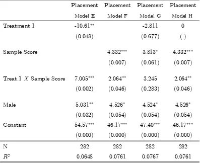
Table 2: Heterogeneous e¤ect - The role of con…dence
Placement Placement Placement Placement
Model E Model F Model G Model H
Treatment 1 -10.61 -2.811 0 (0.048) (0.677) ( )
Sample Score 4.332 3.813 4.332 (0.007) (0.061) (0.007)
Treat.1 X Sample Score 7.005 2.064 3.245 2.064 (0.002) (0.046) (0.283) (0.046)
Male 5.031 4.526 4.524 4.526 (0.032) (0.054) (0.054) (0.054) Constant 54.57 46.17 47.40 46.17
(0.000) (0.000) (0.000) (0.000)
N 282 282 282 282
R2 0.0648 0.0761 0.0767 0.0761
NOTES: The dependent variable is placement (the reported belief that own performance
in the quiz is above the median). Models E-G are OLS regressions. Model H is a
semi-structural estimation imposing the model’s restriction that Treatment1 > 0. P-values in parentheses. p <0:10, p <0:05, p <0:01.
in Table 2. Models E-G are OLS regressions, showing that the interaction term is positive and only insigni…cant when both T reatment 1 and Sample Score are included as regressors. Model H is a semi-structural estimation imposing a model restriction that derives from assuming the presence of control motives. More speci…cally, as highlighted by Proposition 1,
CH > 0 impliesp1 > p2 for all . In accordance with this restriction, we run a constrained
regression imposing that the intercept estimated for treatment 1 must lie weakly above the intercept for treatment 2. The estimation is reported under Model H, which is essentially equivalent to model F given the negative sign of the estimated Treatment-1 coe¢cient in Model G, which is the unrestricted version of model H. The e¤ect of the interaction term becomes signi…cant at the 5% level. The regression analysis with the exclusion of the 3 outliers (who scored zero in the sample questions) is fundamentally unchanged. All things considered, we …nd suggestive but not particularly robust evidence that control motives are increasing in con…dence levels. One must still keep in mind that this is an “out of sample” prediction of our model (it was not built to yield this prediction), that the data is in line with the prediction (and, importantly, does not reject it), and that the sample size of the experiment was intended for the more basic test of p1 > p2:
Note that our prediction that more con…dent individuals in‡ate more for control reasons is unrelated to the Kruger and Dunning (1999)unskilled and unaware e¤ect, which maintains that unskilled people are especially overcon…dent in their beliefs, as this e¤ect is about people’s actual beliefs, not their reports of these beliefs. Moreover, control is not implicated in the Kruger and Dunning experiments, which elicit beliefs in an unincentivized manner.
5.2
Experiment 2
Experiment 2 was run in the same laboratory in Fall 2016. One hundred ninety-six under-graduates participated, drawn again from the University of Amsterdam. No subject took part in both experiments.
The three treatments exhibit basically the same average estimate of pi. In Treatment 1,
with 68 subjects,p1 = 66:2%; in Treatment 2, with 61 subjects,p2 = 67:9%; in Treatment 3,
with 67 subjects,p3 = 66:7%. There are large standard deviations of comparable magnitude
across treatments (16:9, 18:5 and 19:8for Treatments 1 3respectively).
We perform two tests. With the Wilcoxon rank sum (Whitney-Newey) test, the p value for equality of distributions is0:61for Treatments 1 and 2,0:76for treatments 2 and 3, and
and we do not reject equality (pvalue =0:58for Treatments 1 and 2,0:72for Treatments 2 and 3, and 0:88 for Treatments 1 and 3).
These …ndings establish that in the experiment the positive control kick for a favourable bet on self is the same as the negative kick for a bet that the subject will place in the bottom half. They also constitute evidence in favour of the theory, which requires p3 = 12p1+ 12p2;
and is not rejected by the data.
6
Conclusion
Social scientists are interested in people’s beliefs about themselves. One way to elicit these beliefs is simply to ask for them. However, with little at stake, people may provide ready answers that have little connection to their actual beliefs. To counter this possibility, re-searchers have designed payment schemes that reward people for accurately reporting their beliefs. In particular, a variety of payment schemes have been designed so that people maximize their utility of money by reporting their actual beliefs.
However, these schemes remain vulnerable to distortions, as subjects may care about more than money. Our study joins work by Heath and Tversky(1991), Goodie and Young(2007), Burks et al. (2013), Owens, Grossman, and Fackler (2014), and Ewers and Zimmermann
(2015), among others, in determining that non-monetary considerations may lead subjects to overstate their beliefs about themselves under ostensibly incentive compatible mechanisms. In one experiment, using the matching probabilities method, subjects in‡ate their reported beliefs about themselves by7% for control reasons; non-monetary considerations account for at least 27% of what would otherwise be estimated to be overcon…dence.
Our study di¤ers from earlier ones in that we introduce a new design that eliminates the control bias for self-bets. This design can be used in a variety of contexts where control is a factor.
7
Appendix A. Using Sample Score as a proxy for
con-…dence
. While we do not observe true beliefs, the intuition suggests (and our model predicts) that they correlate with reported beliefs, as captur