1694
Stochastic Answer Networks for Machine Reading Comprehension
Xiaodong Liu†, Yelong Shen†, Kevin Duh‡and Jianfeng Gao†
†Microsoft Research, Redmond, WA, USA ‡Johns Hopkins University, Baltimore, MD, USA
†{xiaodl,yeshen,jfgao}@microsoft.com ‡[email protected]
Abstract
We propose a simple yet robuststochastic answer network (SAN) that simulates multi-step reasoning in machine reading
comprehension. Compared to previous
work such as ReasoNet which used rein-forcement learning to determine the num-ber of steps, the unique feature is the use of a kind of stochastic prediction dropout on the answer module (final layer) of the neu-ral network during the training. We show that this simple trick improves robustness and achieves results competitive to the state-of-the-art on the Stanford Question Answering Dataset (SQuAD), the Adver-sarial SQuAD, and the Microsoft MA-chine Reading COmprehension Dataset (MS MARCO).
1 Introduction
Machine reading comprehension (MRC) is a chal-lenging task: the goal is to have machines read a text passage and then answer any question about the passage. This task is an useful benchmark to demonstrate natural language understanding, and also has important applications in e.g. conversa-tional agents and customer service support. It has been hypothesized that difficult MRC problems re-quire some form of multi-step synthesis and rea-soning. For instance, the following example from the MRC dataset SQuAD (Rajpurkar et al., 2016) illustrates the need for synthesis of information across sentences and multiple steps of reasoning:
Q: What collection does the V&A Theator & Performance gallerieshold?
P: The V&A Theator & Performance
gal-leries opened in March 2009. ... They
hold the UK’s biggest national collection of
material about live performance.
To infer the answer (the underlined portion of the passageP), the model needs to first perform coref-erence resolution so that it knows “They” refers “V&A Theator”, then extract the subspan in the direct object corresponding to the answer.
This kind of iterative process can be viewed as a form of multi-step reasoning. Several recent MRC models have embraced this kind of multi-step strategy, where predictions are generated after making multiple passes through the same text and integrating intermediate information in the pro-cess. The first models employed a predetermined fixed number of steps (Hill et al., 2016; Dhingra et al., 2016; Sordoni et al., 2016; Kumar et al., 2015). Later, Shen et al. (2016) proposed using reinforcement learning to dynamically determine the number of steps based on the complexity of the question. Further, Shen et al. (2017) empir-ically showed that dynamic multi-step reasoning outperforms fixed multi-step reasoning, which in turn outperforms single-step reasoning on two dis-tinct MRC datasets (SQuAD and MS MARCO).
predic-st-1 st st+1
x
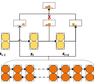
Figure 1: Illustration of “stochastic prediction dropout” in the answer module during training. At each reasoning stept, the model combines mem-ory (bottom row) with hidden statesst−1to
gener-ate a prediction (multinomial distribution). Here, there are three steps and three predictions, but one prediction is dropped and the final result is an av-erage of the remaining distributions.
tion refinements. Stochastic prediction dropout is illustrated in Figure 1.
2 Proposed model: SAN
The machine reading comprehension (MRC)
task as defined here involves a question
Q = {q0, q1, ..., qm−1} and a passage
P = {p0, p1, ..., pn−1} and aims to find an
answer spanA={astart, aend}inP. We assume that the answer exists in the passage P as a contiguous text string. Here,mandndenote the number of tokens in QandP, respectively. The learning algorithm for reading comprehension is to learn a function f(Q, P) → A. The training data is a set of the query, passage and answer tuples< Q, P, A >.
We now describe our model from the ground up. The main contribution of this work is the answer module, but in order to understand what goes into this module, we will start by describing how Q andP are processed by the lower layers. Note the lower layers also have some novel variations that are not used in previous work. As shown in Fig-ure 2, our model contains four different layers to capture different concept of representations. The detailed description of our model is provided as follows.
Lexicon Encoding Layer. The purpose of the first layer is to extract information fromQandP at the word level and normalize for lexical
vari-ants. A typical technique to obtain lexicon embed-ding is concatenation of its word embedembed-ding with other linguistic embedding such as those derived from Part-Of-Speech (POS) tags. For word em-beddings, we use the pre-trained 300-dimensional GloVe vectors (Pennington et al., 2014) for the bothQandP. Following Chen et al. (2017), we use three additional types of linguistic features for each tokenpiin thepassageP:
• 9-dimensional POS tagging embedding for total 56 different types of the POS tags.
• 8-dimensional named-entity recognizer
(NER) embedding for total 18 different types of the NER tags. We utilized small embedding sizes for POS and NER to reduce model size. They mainly serve the role of coarse-grained word clusters.
• A 3-dimensional binary exact match fea-ture defined as fexact match(pi) = I(pi ∈ Q). This checks whether a passage token pi matches the original, lowercase or lemma form of any question token.
• Question enhanced passages word
embed-dings: falign(pi) = Pjγi,jg(GloV e(qj)), where g(·) is a 280-dimensional single layer neural network ReLU(W0x) and
γi,j =
exp(g(GloV e(pj))·g(GloV e(qi)))
P
j0exp(g(GloV e(pi))·g(GloV e(qj0)))
mea-sures the similarity in word embedding space between a token pi in the passage and a to-kenqj in the question. Compared to the ex-actmatching features, these embeddings en-codesoftalignments between similar but not-identical words.
In summary, each tokenpiin the passage is repre-sented as a 600-dimensional vector and each token qj is represented as a 300-dimensional vector.
Due to different dimensions for the passages and questions, in the next layer two different bidirectional LSTM (BiLSTM) (Hochreiter and Schmidhuber, 1997) may be required to encode the contextual information. This, however, in-troduces a large number of parameters. To pre-vent this, we employ an idea inspired by (Vaswani et al., 2017): use two separate two-layer position-wise Feed-Forward Networks (FFN),F F N(x) =
W2ReLU(W1x+b1)+b2, to map both the passage
[image:2.595.112.268.69.206.2]Question Lexicon
Encoding Layer
Document
Word Embedding Surface Feature
Beyoncé is … what religion?
2 Layers Position-Wise FFN
Beyoncé was born ... in a Methodist household.
2 Layers Position-Wise FFN
Beyoncé was born ... in a Methodist household.
2 Layers Position-Wise FFN Contextual
Encoding Layer
Attention Self Attention
2 Layers BiLSTM with Maxout
Memory
Self Attended Sum
GRU
st-1 st st+1
Figure 2:Architecture of the SAN for Reading Comprehension:The first layer is a lexicon encoding layer that maps words to their embeddings independently for the question (left) and the passage (right): this is a concatenation of word embeddings, POS embeddings, etc. followed by a position-wise FFN. The next layer is a context encoding layer, where a BiLSTM is used on the top of the lexicon embedding layer to obtain the context representation for both question and passage. In order to reduce the parameters, a maxout layer is applied on the output of BiLSTM. The third layer is the working memory: First we compute an alignment matrix between the question and passage using an attention mechanism, and use this to derive a question-aware passage representation. Then we concatenate this with the context representation of passage and the word embedding, and employ a self attention layer to re-arrange the information gathered. Finally, we use another LSTM to generate a working memory for the passage. At last, the fourth layer is the answer module, which is a GRU that outputs predictions at each statest.
parameters compared to a BiLSTM. Thus, we ob-tain the final lexicon embeddings for the tokens in Q as a matrix Eq ∈
Rd×m and tokens in P as
Ep ∈Rd×n.
Contextual Encoding Layer. Both passage and question use a shared two-layers BiLSTM as the contextual encoding layer, which projects the lexicon embeddings to contextual embeddings. We concatenate a pre-trained 600-dimensional CoVe vectors1 (McCann et al., 2017) trained on German-English machine translation dataset, with
1https://github.com/salesforce/cove
the aforementioned lexicon embeddings as the fi-nal input of the contextual encoding layer, and also with the output of the first contextual encoding layer as the input of its second encoding layer. To reduce the parameter size, we use a maxout layer (Goodfellow et al., 2013) at each BiLSTM layer to shrink its dimension. By a concatena-tion of the outputs of two BiLSTM layers, we obtain Hq ∈ R2d×m as representation of Q and Hp ∈ R2d×n as representation of P, where dis
the hidden size of the BiLSTM.
generation layer, We construct the working mem-ory, a summary of information from both Q and P. First, a dot-product attention is adopted like in (Vaswani et al., 2017) to measure the similarity between the tokens inQandP. Instead of using a scalar to normalize the scores as in (Vaswani et al., 2017), we use one layer network to transform the contextual information of bothQandP:
C =dropout(fattention( ˆHq,Hˆp))∈Rm×n (1)
C is an attention matrix. Note thatHˆqandHˆpis transformed from Hq and Hp by one layer neu-ral networkReLU(W3x), respectively. Next, we
gather all the information on passages by a sim-ple concatenation of its contextual informationHp and its question-aware representationHq·C:
Up=concat(Hp, HqC)∈R4d×n (2)
Typically, a passage may contain hundred of to-kens, making it hard to learn the long dependen-cies within it. Inspired by (Lin et al., 2017), we apply a self-attended layer to rearrange the infor-mationUpas:
ˆ
Up =Updropdiag(fattention(Up, Up)). (3)
In other words, we first obtain ann×nattention matrix with Up onto itself, apply dropout, then multiply this matrix withUpto obtain an updated
ˆ
Up. Instead of using a penalization term as in (Lin et al., 2017), we dropout the diagonal of the sim-ilarity matrix forcing each token in the passage to align to other tokens rather than itself.
At last, the working memory is generated by us-ing another BiLSTM based on all the information gathered:
M =BiLST M([Up; ˆUp]) (4)
where the semicolon mark ; indicates the vec-tor/matrix concatenation operator.
Answer module. There is a Chinese proverb that says: “wisdom of masses exceeds that of any individual.” Unlike other multi-step reasoning models, which only uses a single output either at the last step or some dynamically determined final step, our answer module employs all the outputs of multiple step reasoning. Intuitively, by applying dropout, it avoids a “step bias problem” (where models places too much emphasis one particular step’s predictions) and forces the model to produce good predictions at every individual step. Further,
during decoding, we reusewisdom of masses in-stead ofindividualto achieve a better result. We call this method “stochastic prediction dropout” because dropout is being applied to the final pre-dictive distributions.
Formally, our answer module will compute over T memory steps and output the answer span. This module is a memory network and has some sim-ilarities to other multi-step reasoning networks: namely, it maintains a state vector, one state per step. At the beginning, the initial state s0 is
the summary of the Q: s0 = PjαjHjq, where
αj =
exp(w4·Hjq)
P
j0exp(w4·Hjq0). At time step t in the
range of {1,2, ..., T −1}, the state is defined by st =GRU(st−1, xt). Here,xtis computed from the previous state st−1 and memory M: xt =
P
jβjMj and βj = sof tmax(st−1W5M).
Fi-nally, a bilinear function is used to find the begin and end point of answer spans at each reasoning stept∈ {0,1, . . . , T −1}.
Ptbegin=sof tmax(stW6M) (5)
Ptend =sof tmax([st;
X
j
Pt,jbeginMj]W7M).
(6) From a pair of begin and end points, the an-swer string can be extracted from the passage. However, rather than output the results (start/end points) from the final step (which is fixed atT−1
as in Memory Networks or dynamically deter-mined as in ReasoNet), we utilize all of theT out-puts by averaging the scores:
Pbegin=avg([P0begin, P1begin, ..., PTbegin−1 ]) (7)
Pend =avg([P0end, P1end, ..., PTend−1]) (8)
Each Ptbegin or Pend
t is a multinomial distribu-tion over {1, . . . , n}, so the average distribution is straightforward to compute.
During training, we apply stochastic dropout to before the above averaging operation. For exam-ple, as illustrated in Figure 1, we randomly delete several steps’ predictions in Equations 7 and 8 so thatPbeginmight beavg([P1begin, P3begin])and Pendmight beavg([P0end, P3end, P4end]). The use of averaged predictions and dropout during train-ing improves robustness.
is dropout at the intermediate node-level, whereas ours is dropout at the final layer-level. Dropout at the node-level prevents correlation between fea-tures. Dropout at the final layer level, where ran-domness is introduced to the averaging of predic-tions, prevents our model from relying exclusively on a particular step to generate correct output. We used a dropout rate of 0.4 in experiments.
3 Experiment Setup
Dataset: We evaluate on the Stanford Question Answering Dataset (SQuAD) (Rajpurkar et al.,
2016). This contains about 23K passages and
100K questions. The passages come from approx-imately 500 Wikipedia articles and the questions and answers are obtained by crowdsourcing. The crowdsourced workers are asked to read a passage (a paragraph), come up with questions, then mark the answer span. All results are on the official de-velopment set, unless otherwise noted.
Two evaluation metrics are used: Exact Match (EM), which measures the percentage of span pre-dictions that matched any one of the ground truth answer exactly, and Macro-averaged F1 score, which measures the average overlap between the prediction and the ground truth answer.
Implementation details: The spaCy tool2 is used to tokenize the both passages and questions, and generate lemma, part-of-speech and named entity tags. We use 2-layer BiLSTM withd= 128
hidden units for both passage and question encod-ing. The mini-batch size is set to 32 and Adamax (Kingma and Ba, 2014) is used as our optimizer. The learning rate is set to 0.002 at first and de-creased by half after every 10 epochs. We set the dropout rate for all the hidden units of LSTM, and the answer module output layer to 0.4. To prevent degenerate output, we ensure that at least one step in the answer module is active during training.
4 Results
The main experimental question we would like to answer is whether the stochastic dropout and av-eraging in the answer module is an effective tech-nique for multi-step reasoning. To do so, we fixed all lower layers and compared different architec-tures for the answer module:
1. Standard 1-step: generate prediction froms0,
the first initial state.
2https://spacy.io
2. 5-step memory network: this is a memory network fixed at 5 steps. We try two variants: the standard variant outputs result from the fi-nal stepsT−1. The averaged variant outputs
results by averaging across all 5 steps, and is like SAN without the stochastic dropout.
3. ReasoNet3: this answer module dynamically decides the number of steps and outputs re-sults conditioned on the final step.
4. SAN: proposed answer module that uses stochastic dropout and prediction averaging.
The main results in terms of EM and F1 are shown in Table 1. We observe that SAN achieves 76.235 EM and 84.056 F1, outperforming all other
models. Standard 1-step model only achieves
75.139 EM and dynamic steps (via ReasoNet) achieves only 75.355 EM. SAN also outperforms a 5-step memory net with averaging, which implies averaging predictions is not the only thing that led to SAN’s superior results; indeed, stochastic pre-diction dropout is an effective technique.
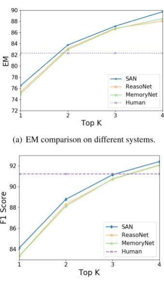
The K-best oracle results is shown in Figure 3. The K-best spans are computed by ordering the spans according the their probabilities Pbegin ×
Pend. We limit K in the range 1 to 4 and then pick the span with the best EM or F1 as oracle. SAN also outperforms the other models in terms of K-best oracle scores. Impressively, these mod-els achieve human performance atK = 2for EM andK= 3for F1.
Finally, we compare our results with other top models in Table 2. Note that all the results in Ta-ble 2 are taken from the published papers. We see that SAN is very competitive in both single and ensemble settings (ranked in second) despite its simplicity. Note that the best-performing model (Peters et al., 2018) used a large-scale language model as an extra contextual embedding, which gave a significant improvement (+4.3% dev F1). We expect significant improvements if we add this to SAN in future work.
3
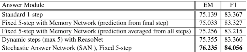
Answer Module EM F1
Standard 1-step 75.139 83.367
Fixed 5-step with Memory Network (prediction from final step) 75.033 83.327
Fixed 5-step with Memory Network (prediction averaged from all steps) 75.256 83.215
Dynamic steps (max 5) with ReasoNet 75.355 83.360
[image:6.595.95.507.61.148.2]Stochastic Answer Network (SAN ), Fixed 5-step 76.235 84.056
Table 1:Main results—Comparison of different answer module architectures. Note that SAN performs best in both Exact Match and F1 metrics.
Ensemble model results: Dev Set (EM/F1) Test Set (EM/F1)
BiDAF + Self Attention + ELMo (Peters et al., 2018) -/- 81.003/87.432
SAN (Ensemble model) 78.619/85.866 79.608/86.496
AIR-FusionNet (Huang et al., 2017) -/- 78.978/86.016
DCN+ (Xiong et al., 2017) -/- 78.852/85.996
M-Reader (Hu et al., 2017) -/- 77.678/84.888
Conductor-net (Liu et al., 2017b) 74.8 / 83.3 76.996/84.630
r-net (Wang et al., 2017) 77.7/83.7 76.9/84.0
ReasoNet++ (Shen et al., 2017) 75.4/82.9 75.0/82.6
Individual model results:
BiDAF + Self Attention + ELMo(Peters et al., 2018) -/- 78.580/85.833
SAN (single model) 76.235/84.056 76.828/84.396
AIR-FusionNet(Huang et al., 2017) 75.3/83.6 75.968/83.900
RaSoR + TR (Salant and Berant, 2017) -/- 75.789/83.261
DCN+(Xiong et al., 2017) 74.5/83.1 75.087/83.081
r-net(Wang et al., 2017) 72.3/80.6 72.3/80.7
ReasoNet++(Shen et al., 2017) 70.8/79.4 70.6/79.36
BiDAF (Seo et al., 2016) 67.7/77.3 68.0/77.3
Human Performance 80.3/90.5 82.3/91.2
Table 2: Test performance on SQuAD. Results are sorted by Test F1.
5 Analysis
5.1 How robust are the results?
We are interested in whether the proposed model is sensitive to different random initial conditions. Table 3 shows the development set scores of SAN trained from initialization with different random seeds. We observe that the SAN results are con-sistently strong regardless of the 10 different ini-tializations. For example, the mean EM score is 76.131 and the lowest EM score is 75.922, both of which still outperform the 75.355 EM of the Dy-namic step ReasoNet in Table 1.4
We are also interested in how sensitive are the results to the number of reasoning steps, which
4Note the Dev EM/F1 scores of ReasoNet in Table 1 do
not match those of ReasoNet++ in Table 2. While the answer module is the same architecture, the lower encoding layers are different.
is a fixed hyper-parameter. Since we are using dropout, a natural question is whether we can ex-tend the number of steps to an extremely large number. Table 4 shows the development set scores for T = 1to T = 10. We observe that there is a gradual improvement as we increaseT = 1 to T = 5, but after 5 steps the improvements have saturated. In fact, the EM/F1 scores drop slightly, but considering that the random initialization re-sults in Table 3 show a standard deviation of 0.142 and a spread of 0.426 (for EM), we believe that the T = 10result does not statistically differ from the T = 5result. In summary, we think it is useful to perform some approximate hyper-parameter tun-ing for the number of steps, but it is not necessary to find the exact optimal value.
(a) EM comparison on different systems.
(b) F1 score comparison on different systems.
Figure 3: K-Best Oracle results
auto-generated adversarial distracting sentences to fool computer systems that are developed to an-swer questions about the passages. For example, AddSent is constructed by adding sentences that look similar to the question, but do not actually contradict the correct answer. AddOneSent is con-structed by appending a random human-approved sentence to the passage.
We evaluate the single SAN model (i.e., the one presented in Table 2) on both AddSent and Ad-dOneSent. The results in Table 5 show that SAN achieves the new state-of-the-art performance and SAN’s superior result is mainly attributed to the multi-step answer module, which leads to signif-icant improvement in F1 score over the Standard 1-step answer module, i.e., +1.2 on AddSent and +0.7 on AddOneSent.
5.2 Is it possible to use different numbers of steps in test vs. train?
For practical deployment scenarios, prediction speed at test time is an important criterion. There-fore, one question is whether SAN can train with, e.g.T = 5steps but test withT = 1steps. Table 6 shows the results of a SAN trained onT = 5steps, but tested with different number of steps. As
ex-Seed# EM F1 Seed# EM F1
Seed 1 76.24 84.06 Seed 6 76.23 83.99
Seed 2 76.30 84.13 Seed 7 76.35 84.09
Seed 3 75.92 83.90 Seed 8 76.07 83.71
Seed 4 76.00 83.95 Seed 9 75.93 83.85
Seed 5 76.12 83.99 Seed 10 76.15 84.11
[image:7.595.94.264.59.353.2]Mean: 76.131, Std. deviation: 0.142 (EM) Mean: 83.977, Std. deviation: 0.126 (F1)
Table 3: Robustness of SAN (5-step) on differ-ent random seeds for initialization: best and worst scores are boldfaced. Note that our official submit is trained on seed 1.
SAN EM F1 SAN EM F1
1 step 75.38 83.29 6 step 75.99 83.72
2 step 75.43 83.41 7 step 76.04 83.92
3 step 75.89 83.57 8 step 76.03 83.82
4 step 75.92 83.85 9 step 75.95 83.75
5 step 76.24 84.06 10 step 76.04 83.89
Table 4: Effect of number of steps: best and worst results are boldfaced.
pected, the results are best whenTmatches during training and test; however, it is important to note
that small numbers of steps T = 1 and T = 2
nevertheless achieve strong results. For example, prediction at T = 1 achieves 75.58, which out-performs a standard 1-step model (75.14 EM) as in Table 1 that has approximate equivalent predic-tion time.
5.3 How does the training time compare?
[image:7.595.314.519.63.179.2]Single model: AddSent AddOneSent
LR (Rajpurkar et al., 2016) 23.2 30.3
SEDT (Liu et al., 2017a) 33.9 44.8
BiDAF (Seo et al., 2016) 34.3 45.7
jNet (Zhang et al., 2017) 37.9 47.0
ReasoNet(Shen et al., 2017) 39.4 50.3
RaSoR(Lee et al., 2016) 39.5 49.5
Mnemonic(Hu et al., 2017) 46.6 56.0
QANet(Yu et al., 2018) 45.2 55.7
Standard 1-step in Table 1 45.4 55.8
[image:8.595.72.298.62.223.2]SAN 46.6 56.5
Table 5: Test performance on the adversarial SQuAD dataset in F1 score.
T = EM F1 T = EM F1
1 75.58 83.86 4 76.12 83.98
2 75.85 83.90 5 76.24 84.06
3 75.98 83.95 10 75.89 83.88
Table 6: Prediction on different stepsT. Note that the SAN model is trained using 5 steps.
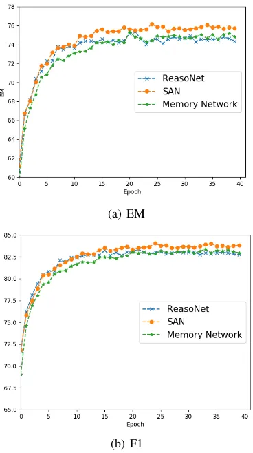
(a) EM
[image:8.595.317.522.62.186.2](b) F1
[image:8.595.86.277.268.328.2]Figure 4: Learning curve measured on Dev set.
Figure 5: Score breakdown by question type.
5.4 How does SAN perform by question type?
To see whether SAN performs well on a particular type of question, we divided the development set by questions type based on their respective
Wh-word, such as “who” and “where”. The score
breakdown by F1 is shown in Figure 5. We ob-serve that SAN seems to outperform other models uniformly across all types. The only exception is the Why questions, but there is too little data to derive strong conclusions.
5.5 Experiments results on MS MARCO
MS MARCO (Nguyen et al., 2016) is a large scale real-word RC dataset which contains 100,100 (100K) queries collected from anonymized user logs from the Bing search engine. The character-istic of MS MARCO is that all the questions are real user queries and passages are extracted from real web documents. For each query, approximate 10 passages are extracted from public web docu-ments. The answers are generated by humans. The data is partitioned into a 82,430 training, a 10,047 development and 9,650 test tuples. The evalua-tion metrics are BLEU(Papineni et al., 2002) and ROUGE-L (Lin, 2004) due to its free-form text answer style. To apply the same RC model, we search for a span in MS MARCO’s passages that maximizes the ROUGE-L score with the raw
free-form answer. It has an upper bound of 93.45
BLEU and 93.82 ROUGE-L on the development set.
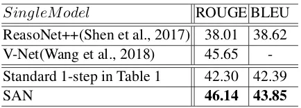
[image:8.595.89.273.377.706.2]ev-SingleM odel ROUGE BLEU ReasoNet++(Shen et al., 2017) 38.01 38.62
V-Net(Wang et al., 2018) 45.65
-Standard 1-step in Table 1 42.30 42.39
[image:9.595.73.290.60.138.2]SAN 46.14 43.85
Table 7:MS MARCO devset results.
ery (Pj, Q) pair, generating J candidate answer spans, one from each passage. Then, we multiply the SAN score of each candidate answer span with its relevance scorer(Pj, Q)assigned by a passage ranker, and output the span with the maximum score as the answer. In our experiments, we use the passage ranker described in (Liu et al., 2018)5. The ranker is trained on the same MS MARCO training data, and achieves 37.1 p@1 on the devel-opment set.
The results in Table 7 show that SAN outper-forms V-Net (Wang et al., 2018) and becomes the new state of the art6.
6 Related Work
The recent big progress on MRC is largely due to the availability of the large-scale datasets (Ra-jpurkar et al., 2016; Nguyen et al., 2016; Richard-son et al., 2013; Hill et al., 2016), since it is possi-ble to train large end-to-end neural network mod-els. In spite of the variety of model structures and attenion types (Bahdanau et al., 2015; Chen et al., 2016; Xiong et al., 2016; Seo et al., 2016; Shen et al., 2017; Wang et al., 2017), a typical neural network MRC model first maps the symbolic rep-resentation of the documents and questions into a neural space, then search answers on top of it. We categorize these models into two groups based on the difference of the answer module: single-step and multi-single-step reasoning. The key difference between the two is what strategies are applied to search the final answers in the neural space.
A single-step model matches the question and document only once and produce the final an-swers. It is simple yet efficient and can be trained using the classical back-propagation algorithm, thus it is adopted by most systems (Chen et al., 2016; Seo et al., 2016; Wang et al., 2017; Liu et al., 2017b; Chen et al., 2017; Weissenborn et al., 2017;
5It is the same model structure as (Liu et al., 2018) by
using softmax over all candidate passages. A simple baseline, TF-IDF, obtains 20.1 p@1 on MS MARCO development.
6The official evaluation on MS MARCO on test is closed,
thus here we only report the results on the development set.
Hu et al., 2017). However, since humans often solve question answering tasks by re-reading and re-digesting the document multiple times before reaching the final answers (this may be based on the complexity of the questions/documents), it is natural to devise an iterative way to find answers as multi-step reasoning.
Pioneered by (Hill et al., 2016; Dhingra et al., 2016; Sordoni et al., 2016; Kumar et al., 2015), who used a predetermined fixed number of rea-soning steps, Shen et al (2016; 2017) showed that multi-step reasoning outperforms single-step ones and dynamic multi-step reasoning further outperforms the fixed multi-step ones on two dis-tinct MRC datasets (SQuAD and MS MARCO). But these models have to be trained using rein-forcement learning methods, e.g., policy gradient, which are tricky to implement due to the instabil-ity issue. Our model is different in that we fix the number of reasoning steps, but perform stochastic dropout to prevent step bias. Further, our model can also be trained by using the back-propagation algorithm, which is simple and yet efficient.
7 Conclusion
We introduce Stochastic Answer Networks
(SAN), a simple yet robust model for machine reading comprehension. The use of stochastic dropout in training and averaging in test at the answer module leads to robust improvements on SQuAD, outperforming both fixed step memory networks and dynamic step ReasoNet. We further empirically analyze the properties of SAN in detail. The model achieves results competitive with the state-of-the-art on the SQuAD leader-board, as well as on the Adversarial SQuAD
and MS MARCO datasets. Due to the strong
connection between the proposed model with memory networks and ReasoNet, we would like to delve into the theoretical link between these models and its training algorithms. Further, we also would like to explore SAN on other tasks, such as text classification and natural language inference for its generalization in the future.
Acknowledgments
References
Dzmitry Bahdanau, Kyunghyun Cho, and Yoshua Ben-gio. 2015. Neural machine translation by jointly learning to align and translate. International Con-ference on Learning Representations (ICLR2015).
Danqi Chen, Jason Bolton, and Christopher D. Man-ning. 2016. A thorough examination of the cnn/daily mail reading comprehension task. In Pro-ceedings of the 54th Annual Meeting of the As-sociation for Computational Linguistics (Volume 1: Long Papers). Association for Computational Linguistics, Berlin, Germany, pages 2358–2367. http://www.aclweb.org/anthology/P16-1223.
Danqi Chen, Adam Fisch, Jason Weston, and Antoine Bordes. 2017. Reading Wikipedia to answer open-domain questions. In Association for Computa-tional Linguistics (ACL).
Bhuwan Dhingra, Hanxiao Liu, William W Cohen, and Ruslan Salakhutdinov. 2016. Gated-attention readers for text comprehension. arXiv preprint arXiv:1606.01549.
Ian J Goodfellow, David Warde-Farley, Mehdi Mirza, Aaron Courville, and Yoshua Bengio. 2013. Maxout networks. arXiv preprint arXiv:1302.4389.
Felix Hill, Antoine Bordes, Sumit Chopra, and Jason Weston. 2016. The goldilocks principle: Reading children’s books with explicit memory representa-tions. ICLR.
Sepp Hochreiter and J¨urgen Schmidhuber. 1997. Long short-term memory. Neural computation
9(8):1735–1780.
Minghao Hu, Yuxing Peng, and Xipeng Qiu. 2017. Mnemonic reader for machine comprehension.
arXiv preprint arXiv:1705.02798.
Hsin-Yuan Huang, Chenguang Zhu, Yelong Shen, and Weizhu Chen. 2017. Fusionnet: Fusing via fully-aware attention with application to machine compre-hension. arXiv preprint arXiv:1711.07341.
Robin Jia and Percy Liang. 2017. Adversarial exam-ples for evaluating reading comprehension systems. In Proceedings of the 2017 Conference on Empiri-cal Methods in Natural Language Processing. pages 2021–2031.
Diederik Kingma and Jimmy Ba. 2014. Adam: A method for stochastic optimization. arXiv preprint arXiv:1412.6980.
Ankit Kumar, Ozan Irsoy, Jonathan Su, James Brad-bury, Robert English, Brian Pierce, Peter Ondruska, Ishaan Gulrajani, and Richard Socher. 2015. Ask me anything: Dynamic memory networks for nat-ural language processing. CoRR abs/1506.07285. http://arxiv.org/abs/1506.07285.
Kenton Lee, Tom Kwiatkowski, Ankur Parikh, and Di-panjan Das. 2016. Learning recurrent span repre-sentations for extractive question answering. arXiv preprint arXiv:1611.01436.
Chin-Yew Lin. 2004. Rouge: A package for automatic evaluation of summaries.
Zhouhan Lin, Minwei Feng, Cicero Nogueira dos San-tos, Mo Yu, Bing Xiang, Bowen Zhou, and Yoshua Bengio. 2017. A structured self-attentive sentence embedding. arXiv preprint arXiv:1703.03130.
Rui Liu, Junjie Hu, Wei Wei, Zi Yang, and Eric Ny-berg. 2017a. Structural embedding of syntactic trees for machine comprehension. InProceedings of the 2017 Conference on Empirical Methods in Natural Language Processing. pages 815–824.
Rui Liu, Wei Wei, Weiguang Mao, and Maria Chik-ina. 2017b. Phase conductor on multi-layered at-tentions for machine comprehension.arXiv preprint arXiv:1710.10504.
Xiaodong Liu, Kevin Duh, and Jianfeng Gao. 2018. Stochastic answer networks for natural language in-ference.arXiv preprint arXiv:1804.07888.
Bryan McCann, James Bradbury, Caiming Xiong, and Richard Socher. 2017. Learned in transla-tion: Contextualized word vectors. arXiv preprint arXiv:1708.00107.
Tri Nguyen, Mir Rosenberg, Xia Song, Jianfeng Gao, Saurabh Tiwary, Rangan Majumder, and Li Deng. 2016. Ms marco: A human generated machine reading comprehension dataset. arXiv preprint arXiv:1611.09268.
Kishore Papineni, Salim Roukos, Todd Ward, and Wei-Jing Zhu. 2002. Bleu: a method for automatic eval-uation of machine translation. In Proceedings of the 40th annual meeting on association for compu-tational linguistics. Association for Computational Linguistics, pages 311–318.
Jeffrey Pennington, Richard Socher, and Christopher Manning. 2014. Glove: Global vectors for word representation. In Proceedings of the 2014 Con-ference on Empirical Methods in Natural Language Processing (EMNLP). Association for Computa-tional Linguistics, Doha, Qatar, pages 1532–1543. http://www.aclweb.org/anthology/D14-1162.
M. E. Peters, M. Neumann, M. Iyyer, M. Gardner, C. Clark, K. Lee, and L. Zettlemoyer. 2018. Deep contextualized word representations. ArXiv e-prints
.
Matthew Richardson, Christopher J.C. Burges, and Erin Renshaw. 2013. MCTest: A challenge dataset for the open-domain machine comprehension of text. InProceedings of the 2013 Conference on Em-pirical Methods in Natural Language Processing. Association for Computational Linguistics, Seattle, Washington, USA, pages 193–203.
S. Salant and J. Berant. 2017. Contextualized Word Representations for Reading Comprehension. ArXiv e-prints.
Minjoon Seo, Aniruddha Kembhavi, Ali Farhadi, and Hannaneh Hajishirzi. 2016. Bidirectional attention flow for machine comprehension. arXiv preprint arXiv:1611.01603.
Yelong Shen, Po-Sen Huang, Jianfeng Gao, and Weizhu Chen. 2016. Reasonet: Learning to stop reading in machine comprehension. arXiv preprint arXiv:1609.05284.
Yelong Shen, Xiaodong Liu, Kevin Duh, and Jianfeng Gao. 2017. An empirical analysis of multiple-turn reasoning strategies in reading comprehension tasks.
arXiv preprint arXiv:1711.03230.
Alessandro Sordoni, Philip Bachman, Adam Trischler, and Yoshua Bengio. 2016. Iterative alternating neu-ral attention for machine reading. arXiv preprint arXiv:1606.02245.
Nitish Srivastava, Geoffrey E Hinton, Alex Krizhevsky, Ilya Sutskever, and Ruslan Salakhutdinov. 2014. Dropout: a simple way to prevent neural networks from overfitting. Journal of Machine Learning Re-search15(1):1929–1958.
Ashish Vaswani, Noam Shazeer, Niki Parmar, Jakob Uszkoreit, Llion Jones, Aidan N Gomez, Lukasz Kaiser, and Illia Polosukhin. 2017. Attention is all you need. arXiv preprint arXiv:1706.03762.
Wenhui Wang, Nan Yang, Furu Wei, Baobao Chang, and Ming Zhou. 2017. Gated self-matching net-works for reading comprehension and question an-swering. InProceedings of the 55th Annual Meet-ing of the Association for Computational LMeet-inguistics (Volume 1: Long Papers). volume 1, pages 189–198.
Y. Wang, K. Liu, J. Liu, W. He, Y. Lyu, H. Wu, S. Li, and H. Wang. 2018. Multi-Passage Ma-chine Reading Comprehension with Cross-Passage Answer Verification.ArXiv e-prints.
Dirk Weissenborn, Georg Wiese, and Laura Seiffe. 2017. Fastqa: A simple and efficient neural ar-chitecture for question answering. arXiv preprint arXiv:1703.04816.
Caiming Xiong, Victor Zhong, and Richard Socher. 2016. Dynamic coattention networks for question answering. arXiv preprint arXiv:1611.01604.
Caiming Xiong, Victor Zhong, and Richard Socher. 2017. Dcn+: Mixed objective and deep residual coattention for question answering. arXiv preprint arXiv:1711.00106.
Adams Wei Yu, David Dohan, Minh-Thang Luong, Rui Zhao, Kai Chen, Mohammad Norouzi, and Quoc V. Le. 2018. Qanet: Combining local convolution with global self-attention for reading comprehension.