380
Evolutionary Data Measures: Understanding the Difficulty of Text
Classification Tasks
Edward Collins
Wluper Ltd. London, United Kingdom
Nikolai Rozanov
Wluper Ltd. London, United Kingdom
Bingbing Zhang
Wluper Ltd. London, United Kingdom
Abstract
Classification tasks are usually analysed and improved through new model architectures or hyperparameter optimisation but the underly-ing properties of datasets are discovered on an ad-hoc basis as errors occur. However, under-standing the properties of the data is crucial in perfecting models. In this paper we anal-yse exactly which characteristics of a dataset best determine how difficult that dataset is for the task of text classification. We then propose an intuitive measure of difficulty for text clas-sification datasets which is simple and fast to calculate. We show that this measure gener-alises to unseen data by comparing it to state-of-the-art datasets and results. This measure can be used to analyse the precise source of errors in a dataset and allows fast estimation of how difficult a dataset is to learn. We searched for this measure by training 12 clas-sical and neural network based models on 78 real-world datasets, then use a genetic algo-rithm to discover the best measure of difficulty. Our difficulty-calculating code1 and datasets2 are publicly available.
1 Introduction
If a machine learning (ML) model is trained on a dataset then the same machine learning model on the same dataset but with more granular labels will frequently have lower performance scores than the original model (see results inZhang et al.(2015);
Socher et al. (2013a); Yogatama et al. (2017);
Joulin et al. (2016); Xiao and Cho (2016); Con-neau et al. (2017)). Adding more granularity to labels makes the dataset harder to learn - it in-creases the dataset’s difficulty. It is obvious that some datasets are more difficult for learning mod-els than others, but is it possible to quantify this
1
https://github.com/Wluper/edm 2http://data.wluper.com
difficulty? In order to do so, it would be neces-sary to understand exactly what characteristics of a dataset are good indicators of how well models will perform on it so that these could be combined into a single measure of difficulty.
Such a difficulty measure would be useful as an analysis tool and as a performance estimator. As an analysis tool, it would highlight precisely what is causing difficulty in a dataset, reducing the time practitioners need spend analysing their data. As a performance estimator, when practitioners ap-proach new datasets they would be able to use this measure to predict how well models are likely to perform on the dataset.
The complexity of datasets for ML has been previously examined (Ho and Basu, 2002; Man-silla and Ho, 2004; Bernad´o-Mansilla and Ho,
2005;Maci et al.,2008), but these works focused on analysing feature space data ∈ IRn. These methods do not easily apply to natural language, because they would require the language be em-bedded into feature space in some way, for exam-ple with a word embedding model which intro-duces a dependency on the model used. We ex-tend previous notions of difficulty to English lan-guage text classification, an important component of natural language processing (NLP) applicable to tasks such as sentiment analysis, news cate-gorisation and automatic summarisation (Socher et al.,2013a;Antonellis et al.,2006;Collins et al.,
2017). All of our recommended calculations de-pend only on counting the words in a dataset.
1.1 Related Work
this work because it can be reduced with proper data cleaning and is not a part of the true signal of the dataset. We identified four other areas of potential difficulty which we attempt to measure:
Class Interference. Text classification tasks to predict the 1 - 5 star rating of a review are more difficult than predicting whether a review is posi-tive or negaposi-tive (Zhang et al.,2015;Socher et al.,
2013a;Yogatama et al.,2017;Joulin et al.,2016;
Xiao and Cho,2016;Conneau et al.,2017), as re-views given four stars share many features with those given five stars. Gupta et al. (2014) de-scribe how as the number of classes in a dataset increases, so does the potential for ”confusabil-ity” where it becomes difficult to tell classes apart, therefore making a dataset more difficult. Previous work has mostly focused on this confusability - or class interference - as a source of difficulty in ma-chine learning tasks (Bernad´o-Mansilla and Ho,
2005;Ho and Basu, 2000,2002;Elizondo et al.,
2009; Mansilla and Ho, 2004), a common tech-nique being to compute a minimum spanning tree on the data and count the number of edges which link different classes.
Class Diversity. Class diversity provides infor-mation about the composition of a dataset by mea-suring the relative abundances of different classes (Shannon,2001). Intuitively, it gives a measure of how well a model could do on a dataset without examining any data items and always predicting the most abundant class. Datasets with a single overwhelming class are easy to achieve high accu-racies on by always predicting the most abundant class. A measure of diversity is one feature used byBingel and Søgaard(2017) to identify datasets which would benefit from multi-task learning.
Class Balance. Unbalanced classes are a known problem in machine learning (Chawla et al.,2004,
2002), particularly if classes are not easily separa-ble (Japkowicz, 2000). Underrepresented classes are more difficult to learn because models are not exposed to them as often.
Data Complexity. Humans find some pieces of text more difficult to comprehend than others. How difficult a piece of text is to read can be calculated automatically using measures such as those proposed byMc Laughlin(1969);Senter and Smith(1967);Kincaid et al.(1975). If a piece of text is more difficult for a human to read and
un-derstand, the same may be true for an ML model.
2 Method
We used 78 text classification datasets and trained 12 different ML algorithms on each of the datasets for a total of 936 models trained. The highest achieved macro F1 score (Powers, 2011), on the test set for each model was recorded. Macro F1 score is used because it is valid under imbalanced classes. We then calculated 48 different statis-tics which attempt to measure our four hypothe-sised areas of difficulty for each dataset. We then needed to discover which statistic or combination thereof correlated with model F1 scores.
We wanted the discovered difficulty measure to be useful as an analysis tool, so we enforced a re-striction that the difficulty measure should be com-posed only by summation, without weighting the constituent statistics. This meant that each diffi-culty measure could be used as an analysis tool by examining its components and comparing them to the mean across all datasets.
Each difficulty measure was represented as a bi-nary vector of length 48 - one bit for each statistic - each bit being 1 if that statistic was used in the difficulty measure. We therefore had248possible different difficulty measures that may have corre-lated with model score and needed to search this space efficiently.
Genetic algorithms are biologically inspired search algorithms and are good at searching large spaces efficiently (Whitley,1994). They maintain a population of candidate difficulty measures and combine them based on their ”fitness” - how well they correlate with model scores - so that each ”parent” can pass on pieces of information about the search space (Jiao and Wang,2000). Using a genetic algorithm, we efficiently discovered which of the possible combinations of statistics corre-lated with model performance.
2.1 Datasets
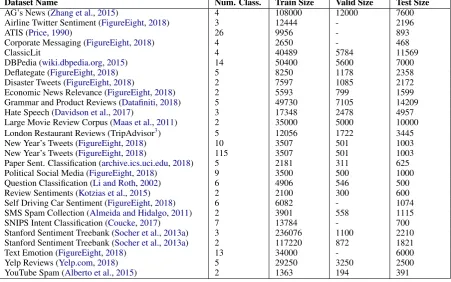
We gathered 27 real-world text classification datasets from public sources, summarised in Table
1; full descriptions are in AppendixA.
Dataset Name Num. Class. Train Size Valid Size Test Size
AG’s News (Zhang et al.,2015) 4 108000 12000 7600
Airline Twitter Sentiment (FigureEight,2018) 3 12444 - 2196
ATIS (Price,1990) 26 9956 - 893
Corporate Messaging (FigureEight,2018) 4 2650 - 468
ClassicLit 4 40489 5784 11569
DBPedia (wiki.dbpedia.org,2015) 14 50400 5600 7000
Deflategate (FigureEight,2018) 5 8250 1178 2358
Disaster Tweets (FigureEight,2018) 2 7597 1085 2172
Economic News Relevance (FigureEight,2018) 2 5593 799 1599
Grammar and Product Reviews (Datafiniti,2018) 5 49730 7105 14209
Hate Speech (Davidson et al.,2017) 3 17348 2478 4957
Large Movie Review Corpus (Maas et al.,2011) 2 35000 5000 10000
London Restaurant Reviews (TripAdvisor3) 5 12056 1722 3445
New Year’s Tweets (FigureEight,2018) 10 3507 501 1003
New Year’s Tweets (FigureEight,2018) 115 3507 501 1003
Paper Sent. Classification (archive.ics.uci.edu,2018) 5 2181 311 625
Political Social Media (FigureEight,2018) 9 3500 500 1000
Question Classification (Li and Roth,2002) 6 4906 546 500
Review Sentiments (Kotzias et al.,2015) 2 2100 300 600
Self Driving Car Sentiment (FigureEight,2018) 6 6082 - 1074
SMS Spam Collection (Almeida and Hidalgo,2011) 2 3901 558 1115
SNIPS Intent Classification (Coucke,2017) 7 13784 - 700
Stanford Sentiment Treebank (Socher et al.,2013a) 3 236076 1100 2210 Stanford Sentiment Treebank (Socher et al.,2013a) 2 117220 872 1821
Text Emotion (FigureEight,2018) 13 34000 - 6000
Yelp Reviews (Yelp.com,2018) 5 29250 3250 2500
[image:3.595.74.526.65.347.2]YouTube Spam (Alberto et al.,2015) 2 1363 194 391
Table 1: The 27 different publicly available datasets we gathered with references.
two different datasets of tweets, so that the classes would not be trivially distinguishable - there is no dataset to classify text as either a tweet or Shake-speare for example as this would be too easy for models. The full list of combined datasets is in AppendixA.2.
Our datasets focus on short text classification by limiting each data item to 100 words. We demon-strate that the difficulty measure we discover with this setup generalises to longer text classification in Section 3.1. All datasets were lowercase with no punctuation. For datasets with no validation set, 15% of the training set was randomly sampled as a validation set at runtime.
2.2 Dataset Statistics
We calculated 12 distinct statistics with differ-ent n-gram sizes to produce 48 statistics of each dataset. These statistics are designed to increase in value as difficulty increases. The 12 statistics are described here and a listing of the full 48 is in Ap-pendixBin Table5. We used n-gram sizes from unigrams up to 5-grams and recorded the average of each statistic over all n-gram sizes. All bility distributions were count-based - the proba-bility of a particular n-gram / class / character was the count of occurrences of that particular entity
divided by the total count of all entities.
2.2.1 Class Diversity
We recorded the Shannon Diversity Index and its normalised variant the Shannon Equitability (Shannon,2001) using the count-based probabil-ity distribution of classes described above.
2.2.2 Class Balance
We propose a simple measure of class imbalance:
Imbal=
C
X
c=1
1
C − nc TDAT A
(1)
C is the total number of classes, nc is the count
of items in classcandTDAT Ais the total number
of data points. This statistic is 0 if there are an equal number of data points in every class and the upper bound is 2 1− 1
C
and is achieved when one class has all the data points - a proof is given in AppendixB.2.
2.2.3 Class Interference
Hellinger Similarity One minus both the aver-age and minimum Hellinger Distance (Le Cam and Yang, 2012) between each pair of classes. Hellinger Distance is 0 if two probability distri-butions are identical so we subtract this from 1 to give a higher score when two classes are sim-ilar giving the Hellinger Simsim-ilarity. One minus the minimum Hellinger Distance is the maximum Hellinger Similarity between classes.
Top N-Gram Interference Average Jaccard similarity (Jaccard, 1912) between the set of the top 10 most frequent n-grams from each class. N-grams entirely composed of stopwords were ig-nored.
Mutual Information Average mutual informa-tion (Cover and Thomas,2012) score between the set of the top 10 most frequent n-grams from each class. N-grams entirely composed of stopwords were ignored.
2.2.4 Data Complexity
Distinct n-grams : Total n-grams Count of dis-tinct n-grams in a dataset divided by the total num-ber of grams. Score of 1 indicates that each n-gram occurs once in the dataset.
Inverse Flesch Reading Ease The Flesch Read-ing Ease (FRE) formula grades text from 100 to 0, 100 indicating most readable and 0 indicating dif-ficult to read (Kincaid et al.,1975). We take the reciprocal of this measure.
N-Gram and Character Diversity Using the Shannon Index and Equitability described by
Shannon(2001) we calculate the diversity and eq-uitability of n-grams and characters. Probability distributions are count-based as described at the start of this section.
2.3 Models
To ensure that any discovered measures did not depend on which model was used (i.e. that they were model agnostic), we trained 12 models on ev-ery dataset. The models are summarised in Table
2. Hyperparameters were not optimised and were identical across all datasets. Specific implemen-tation details of the models are described in Ap-pendixC. Models were evaluated using the macro F1-Score. These models used three different rep-resentations of text to learn from to ensure that the discovered difficulty measure did not depend on the representation. These are:
Word Embeddings Our neural network mod-els excluding the Convolutional Neural Net-work (CNN) used 128-dimensional FastText ( Bo-janowski et al., 2016) embeddings trained on the One Billion Word corpus (Chelba et al., 2013) which provided an open vocabulary across the datasets.
Term Frequency Inverse Document Frequency (tf-idf) Our classical machine learning mod-els represented each data item as a tf-idf vector (Ramos et al., 2003). This vector has one entry for each word in the vocab and if a word occurs in a data item, then that position in the vector is the word’s tf-idf score.
Characters Our CNN, inspired by Zhang et al.
(2015), sees only the characters of each data item. Each character is assigned an ID and the list of IDs is fed into the network.
2.4 Genetic Algorithm
The genetic algorithm maintains a population of candidate difficulty measures, each being a binary vector of length 48 (see start of Method section). At each time step, it will evaluate each member of the population using afitness function. It will then select pairs of parents based on their fitness, and performcrossoverandmutationon each pair to produce a new child difficulty measure, which is added to the next population. This process is iterated until the fitness in the population no longer improves.
Population The genetic algorithm is non-randomly initialised with the 48 statistics de-scribed in Section 2.2 - each one is a difficulty measure composed of a single statistic. 400 pairs of parents are sampled with replacement from each population, so populations after this first time step will consist of 200 candidate measures. The probability of a measure being selected as a parent is proportional to its fitness.
Word Embedding Based tf-idf Based Character Based
LSTM-RNN Adaboost 3 layer CNN
GRU-RNN Gaussian Naive Bayes (GNB)
-Bidirectional LSTM-RNN 5-Nearest Neighbors
-Bidirectional GRU-RNN (Multinomial) Logistic Regression
-Multilayer Perceptron (MLP) Random Forest
-- Support Vector Machine
-Table 2: Models summary organised by which input type they use.
so if it is high then correlation must be high for every model.
Crossover and Mutation To produce a new dif-ficulty measure from two parents, the constituent statistics of each parent are randomly intermin-gled, allowing each parent to pass on information about the search space. This is done in the follow-ing way: for each of the 48 statistics, one of the two parents is randomly selected and if the parent uses that statistic, the child also does. This pro-duces a child which has features of both parents. To introduce more stochasticity to the process and ensure that the algorithm does not get trapped in a local minima of fitness, the child is mutated. Mutation is performed by randomly adding or tak-ing away each of the 48 statistics with probability 0.01. After this process, the child difficulty mea-sure is added to the new population.
Training The process of calculating fitness, se-lecting parents and creating child difficulty mea-sures is iterated until there has been no improve-ment in fitness for 15 generations. Due to the stochasticity in the process, we run the whole evo-lution 50 times. We run 11 different variants of this evolution, leaving out different statistics of the dataset each time to test which are most impor-tant in finding a good difficulty measure, in total running 550 evolutions. Training time is fast, av-eraging 79 seconds per evolution with a standard deviation of 25 seconds, determined over 50 runs of the algorithm on a single CPU.
3 Results and Discussion
The four hypothesized areas of difficulty - Class Diversity, Balance and Interference and Data Complexity - combined give a model agnostic measure of difficulty. All runs of the genetic al-gorithm produced different combinations of statis-tics which had strong negative correlation with model scores on the 78 datasets. The mean cor-relation was −0.8795 and the standard deviation
was0.0046. Of the measures found through evo-lution we present two of particular interest:
1. D1: Distinct Unigrams : Total Unigrams + Class Imbalance + Class Diversity + Top 5-Gram Interference + Maximum Unigram Hellinger Similarity + Unigram Mutual Info. This measure achieves the highest correlation of all measures at−0.8845.
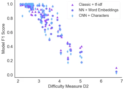
[image:5.595.74.528.62.133.2]2. D2: Distinct Unigrams : Total Unigrams + Class Imbalance + Class Diversity + Max-imum Unigram Hellinger Similarity + Uni-gram Mutual Info. This measure is the short-est measure which achieves a higher correla-tion than the mean, at−0.8814. This measure is plotted against model F1 scores in Figure1.
Figure 1: Model F1 scores against difficulty measure D2 for each of the three input types.
[image:5.595.312.518.439.589.2]Model AG Sogou Yelp P.
Yelp F.
DBP Yah A.
Amz. P.
Amz. F.
Corr.
D2 3.29 3.77 3.59 4.42 3.50 4.51 3.29 4.32
-char-CNN (Zhang et al.,2015) 87.2 95.1 94.7 62 98.3 71.2l 95.1 59.6 -0.86 Bag of Words (Zhang et al.,
2015)
88.8 92.9 92.2 57.9 96.6 68.9 90.4 54.6 -0.87
Discrim. LSTM (Yogatama et al.,2017)
92.1 94.9 92.6 59.6 98.7 73.7 - - -0.87
Genertv. LSTM (Yogatama et al.,2017)
90.6 90.3 88.2 52.7 95.4 69.3 - - -0.88
Kneser-Ney Bayes (Yogatama et al.,2017)
89.3 94.6 81.8 41.7 95.4 69.3 - - -0.79
FastText Lin. Class. (Joulin et al.,2016)
91.5 93.9 93.8 60.4 98.1 72 91.2 55.8 -0.86
Char CRNN (Xiao and Cho,
2016)
91.4 95.2 94.5 61.8 98.6 71.7 94.1 59.2 -0.88
VDCNN (Conneau et al.,2017) 91.3 96.8 95.7 64.7 98.7 73.4 95.7 63 -0.88
Harmonic Mean -0.86
Table 3: Difficulty measure D2 compared to recent results from papers on large-scale text classification. The correlation column reports the correlation between difficulty measure D2 and the model scores for that row.
3.1 Does it Generalise?
A difficulty measure is useful as an analysis and performance estimation tool if it is model agnos-tic and provides an accurate difficulty estimate on unseen datasets.
When running the evolution, the F1 scores of our character-level CNN were not observed by the genetic algorithm. If the discovered difficulty measure still correlated with the CNN’s scores de-spite never having seen them during evolution, it is more likely to be model agnostic. The CNN has a different model architecture to the other mod-els and has a different input type which encodes no prior knowledge (as word embeddings do) or contextual information about the dataset (as tf-idf does). D1 has a correlation of−0.9010with the CNN and D2 has a correlation of−0.8974which suggests that both of our presented measures do not depend on what model was used.
One of the limitations of our method was that our models never saw text that was longer than 100 words and were never trained on any very large datasets (i.e.>1 million data points). We also per-formed no hyperparameter optimisation and did not use state-of-the-art models. To test whether our measure generalises to large datasets with text longer than 100 words, we compared it to some recent state-of-the-art results in text classification using the eight datasets described byZhang et al.
(2015). These results are presented in Table3and highlight several important findings.
The Difficulty Measure Generalises to Very Large Datasets and Long Data Items. The
smallest of the eight datasets described byZhang et al. (2015) has 120 000 data points and the largest has 3.6 million. As D2 still has a strong negative correlation with model score on these datasets, it seems to generalise to large datasets. Furthermore, these large datasets do not have an upper limit of data item length (the mean data item length in Yahoo Answers is 520 words), yet D2 still has strong negative correlation with model score, showing that it does not depend on data item length.
The Difficulty Measure is Model and Input Type Agnostic. The state-of-the-art models pre-sented in Table 3 have undergone hyperparame-ter optimisation and use different input types in-cluding per-word learned embeddings (Yogatama et al.,2017), n-grams, characters and n-gram em-beddings (Joulin et al., 2016). As D2 still has a strong negative correlation with these models’ scores, we can conclude that it has accurately mea-sured the difficulty of a dataset in a way that is useful regardless of which model is used.
The Difficulty Measure Lacks Precision. The average score achieved on the Yahoo Answers dataset is69.9%and its difficulty is4.51. The av-erage score achieved on Yelp Full is56.8%,13.1%
scores> 4, whereas the five datasets with scores
> 90% all have difficulty scores between 3 and 4. This indicates that the difficulty measure in its current incarnation may be more effective at as-signing a class of difficulty to datasets, rather than a regression-like value.
3.2 Difficulty Measure as an Analysis Tool
Statistic Mean Sigma
Distinct Words : Total Words 0.0666 0.0528
Class Imbalance 0.503 0.365
Class Diversity 0.905 0.759
Max. Unigram Hellinger Similarity 0.554 0.165 Top Unigram Mutual Info 1.23 0.430
Table 4: Means and standard deviations of the con-stituent statistics of difficulty measure D2 across the 78 datasets from this paper and the eight datasets from
Zhang et al.(2015).
As our difficulty measure has no dependence on learned weightings or complex combinations of statistics - only addition - it can be used to analyse the sources of difficulty in a dataset directly. To demonstrate, consider the following dataset:
Stanford Sentiment Treebank Binary Classifi-cation (SST 2) (Socher et al.,2013b) SST is a dataset of movie reviews for which the task is to classify the sentiment of each review. The current state-of-the-art accuracy is91.8%(Radford et al.,
[image:7.595.76.286.501.653.2]2017).
Figure 2: Constituents of difficulty measure D2 for SST, compared to the mean across all datasets.
Figure2shows the values of the constituent statis-tics of difficulty measure D2 for SST and the mean values across all datasets. The mean (right bar)
also includes an error bar showing the standard de-viation of statistic values. The exact values of the means and standard deviations for each statistic in measure D2 are shown in Table4.
Figure2shows that for SST 2 the Mutual Infor-mation is more than one standard deviation higher than the mean. A high mutual information score indicates that reviews have both positive and neg-ative features. For example, consider this review:
”de niro and mcdormand give solid performances but their screen time is sabotaged by the story s in-ability to create interest”which is labelled ”pos-itive”. There is a positive feature referring to the actors’ performances and a negative one referring to the plot. A solution to this would be to treat the classification as a multi-label problem where each item can have more than one class, although this would require that the data be relabelled by hand. An alternate solution would be to split reviews like this into two separate ones: one with the positive component and one with the negative.
Furthermore, Figure 2 shows that the Max. Hellinger Similarity is higher than average for SST 2, indicating that the two classes use simi-lar words. Sarcastic reviews use positive words to convey a negative sentiment (Maynard and Green-wood, 2014) and could contribute to this higher value, as could mislabelled items of data. Both of these things portray one class with features of the other - sarcasm by using positive words with a negative tone and noise because positive exam-ples are labelled as negative and vice versa. This kind of difficulty can be most effectively reduced by filtering noise (Smith et al.,2014).
3.3 The Important Areas of Difficulty
We hypothesized that the difficulty of a dataset would be determined by four areas not including noise: Class Diversity, Class Balance, Class Inter-ference and Text Complexity. We performed mul-tiple runs of the genetic algorithm, leaving statis-tics out each time to test which were most impor-tant in finding a good difficulty measure which re-sulted in the following findings:
No Single Characteristic Describes Difficulty When the Class Diversity statistic was left out of evolution, the highest achieved correlation was
−0.806, 9% lower than D1 and D2. However, on its own Class Diversity had a correlation of
−0.644 with model performance. Clearly, Class Diversity is necessary but not sufficient to estimate dataset difficulty. Furthermore, when all measures of Class Diversity and Balance were excluded, the highest achieved correlation was−0.733and when all measures of Class Interference were ex-cluded the best correlation was −0.727. These three expected areas of difficulty - Class Diversity, Balance and Interference - must all be measured to get an accurate estimate of difficulty because ex-cluding any of them significantly damages the cor-relation that can be found. Corcor-relations for each individual statistic are in Table6, in AppendixD.
Data Complexity Has Little Affect on Diffi-culty Excluding all measures of Data Complex-ity from evolution yielded an average correlation of−0.869, only1%lower than the average when all statistics were included. Furthermore, the only measure of Data Complexity present in D1 and D2 is Distinct Words : Total Words which has a mean value of0.067and therefore contributes very little to the difficulty measure. This shows that while Data Complexity is necessary to achieve top cor-relation, its significance is minimal in comparison to the other areas of difficulty.
3.4 Error Analysis
3.4.1 Overpowering Class Diversity
When a dataset has a large number of balanced classes, then Class Diversity dominates the mea-sure. This means that the difficulty measure is not a useful performance estimator for such datasets.
To illustrate this, we created several fake datasets with 1000, 100, 50 and 25 classes. Each dataset had 1000 copies of the same randomly generated string in each class. It was easy for
mod-els to overfit and score a 100% F1 score on these fake datasets.
For the 1000-class fake data, Class Diversity is
6.91, which by our difficulty measure would indi-cate that the dataset is extremely difficult. How-ever, all models easily achieve a 100% F1 score. By testing on these fake datasets, we found that the limit for the number of classes before Class Diver-sity dominates the difficulty measure and renders it inaccurate is approximately 25. Any datasets with more than 25 classes with an approximately equal number of items per class will be predicted as difficult regardless of whether they actually are because of this diversity measure.
Datasets with more than 25unbalancedclasses are still measured accurately. For example, the ATIS dataset (Price,1990) has 26 classes but be-cause some of them have only 1 or 2 data items, it is not dominated by Class Diversity. Even when the difficulty measure is dominated by Class Di-versity, examining the components of the difficulty measure independently would still be useful as an analysis tool.
3.4.2 Exclusion of Useful Statistics
One of our datasets of New Year’s Resolution Tweets has 115 classes but only 3507 data points (FigureEight, 2018). An ML practitioner knows from the number of classes and data points alone that this is likely to be a difficult dataset for an ML model.
Our genetic algorithm, based on an unweighted, linear sum, cannot take statistics like data size into account currently because they do not have a con-venient range of values; the number of data points in a dataset can vary from several hundred to sev-eral million. However, the information is still use-ful to practitioners in diagnosing the difficulty of a dataset.
3.5 How to Reduce the Difficulty Measure
Here we present some general guidelines on how the four areas of difficulty can be reduced.
Class Diversity can only be sensibly reduced by lowering the number of classes, for example by grouping classes under superclasses. In academic settings where this is not possible, hierarchical learning allows grouping of classes but will pro-duce granular labels at the lowest level (Kowsari et al.,2017). Ensuring a large quantity of data in each class will also help models to better learn the features of each class.
Class Interference is influenced by the amount of noise in the data and linguistic phenomena like sarcasm. It can also be affected by the way the data is labelled, for example as shown in Section 3.2
where SST has data points with both positive and negative features but only a single label. Filtering noise, restructuring or relabelling ambiguous data points and detecting phenomena like sarcasm will help to reduce class interference. Easily confused classes can also be grouped under one superclass if practitioners are willing to sacrifice granularity to gain performance.
Class Imbalance can be addressed with data augmentation such as thesaurus based methods (Zhang et al.,2015) or word embedding perturba-tion (Zhang and Yang, 2018). Under- and over-sampling can also be utilised (Chawla et al.,2002) or more data gathered. Another option is transfer learning where knowledge from high data domains can be transferred to those with little data (Jaech et al.,2016).
Data Complexity can be managed with large amounts of data. This need not necessarily be la-belled - unsupervised pre-training can help mod-els understand the form of complex data before attempting to use it (Halevy et al., 2009). Cur-riculum learning may also have a similar effect to pre-training (Bengio et al.,2009).
3.6 Other Applications of the Measure
Model Selection Once the difficulty of a dataset has been calculated, a practitioner can use this to decide whether they need a complex or simple model to learn the data.
Performance Checking and Prediction Practi-tioners will be able to compare the results their models get to the scores of other models on datasets of an equivalent difficulty. If their mod-els achieve lower results than what is expected
ac-cording to the difficulty measure, then this could indicate a problem with the model.
4 Conclusion
When their models do not achieve good results, ML practitioners could potentially calculate thou-sands of statistics to see what aspects of their datasets are stopping their models from learning. Given this, how do practitioners tell which statis-tics are the most useful to calculate? Which ones will tell them the most? What changes could they make which will produce the biggest increase in model performance?
In this work, we have presented two measures of text classification dataset difficulty which can be used as analysis tools and performance estimators. We have shown that these measures generalise to unseen datasets. Our recommended measure can be calculated simply by counting the words and labels of a dataset and is formed by adding five different, unweighted statistics together. As the difficulty measure is an unweighted sum, its com-ponents can be examined individually to analyse the sources of difficulty in a dataset.
There are two main benefits to this difficulty measure. Firstly, it will reduce the time that practitioners need to spend analysing their data in order to improve model scores. As we have demonstrated which statistics are most indicative of dataset difficulty, practitioners need only calcu-late these to discover the sources of difficulty in their data. Secondly, the difficulty measure can be used as a performance estimator. When practi-tioners approach new tasks they need only calcu-late these simple statistics in order to estimate how well models are likely to perform.
Furthermore, this work has shown that for text classification the areas of Class Diversity, Balance and Interference are essential to measure in order to understand difficulty. Data Complexity is also important, but to a lesser extent.
References
T´ulio C Alberto, Johannes V Lochter, and Tiago A Almeida. 2015. Tubespam: Comment spam filter-ing on youtube. InMachine Learning and Applica-tions (ICMLA), 2015 IEEE 14th International Con-ference on, pages 138–143. IEEE. [Online; accessed 22-Feb-2018].
Tiago A. Almeida and Jos Mara Gmez Hidalgo. 2011. Sms spam collection v. 1. [Online; accessed 25-Feb-2018].
Ioannis Antonellis, Christos Bouras, and Vassilis Poulopoulos. 2006. Personalized news categoriza-tion through scalable text classificacategoriza-tion. In Asia-Pacific Web Conference, pages 391–401. Springer.
archive.ics.uci.edu. 2018. Sentence classification data
set. https://archive.ics.uci.edu/ml/
datasets/Sentence+Classification. [Online; accessed 20-Feb-2018].
Jacob Benesty, Jingdong Chen, Yiteng Huang, and Is-rael Cohen. 2009. Pearson correlation coefficient. InNoise reduction in speech processing, pages 1–4. Springer.
Yoshua Bengio, J´erˆome Louradour, Ronan Collobert, and Jason Weston. 2009. Curriculum learning. In
Proceedings of the 26th annual international
con-ference on machine learning, pages 41–48. ACM.
Ester Bernad´o-Mansilla and Tin Kam Ho. 2005. Do-main of competence of xcs classifier system in com-plexity measurement space. IEEE Transactions on
Evolutionary Computation, 9(1):82–104.
Joachim Bingel and Anders Søgaard. 2017. Identi-fying beneficial task relations for multi-task learn-ing in deep neural networks. arXiv preprint
arXiv:1702.08303.
Piotr Bojanowski, Edouard Grave, Armand Joulin, and Tomas Mikolov. 2016. Enriching word vec-tors with subword information. arXiv preprint
arXiv:1607.04606.
Carla E Brodley and Mark A Friedl. 1999. Identifying mislabeled training data. Journal of artificial intel-ligence research, 11:131–167.
Nitesh V Chawla, Kevin W Bowyer, Lawrence O Hall, and W Philip Kegelmeyer. 2002. Smote: synthetic minority over-sampling technique. Journal of artifi-cial intelligence research, 16:321–357.
Nitesh V Chawla, Nathalie Japkowicz, and Aleksander Kotcz. 2004. Special issue on learning from imbal-anced data sets. ACM Sigkdd Explorations Newslet-ter, 6(1):1–6.
Ciprian Chelba, Tomas Mikolov, Mike Schuster, Qi Ge, Thorsten Brants, Phillipp Koehn, and Tony Robin-son. 2013. One billion word benchmark for measur-ing progress in statistical language modelmeasur-ing. arXiv preprint arXiv:1312.3005.
Kyunghyun Cho, Bart Van Merri¨enboer, Caglar Gul-cehre, Dzmitry Bahdanau, Fethi Bougares, Holger Schwenk, and Yoshua Bengio. 2014. Learning phrase representations using rnn encoder-decoder for statistical machine translation. arXiv preprint arXiv:1406.1078.
Ed Collins, Isabelle Augenstein, and Sebastian Riedel. 2017. A supervised approach to extractive sum-marisation of scientific papers. In Proceedings of the 21st Conference on Computational Natural
Lan-guage Learning (CoNLL 2017), pages 195–205.
Alexis Conneau, Holger Schwenk, Lo¨ıc Barrault, and Yann Lecun. 2017. Very deep convolutional net-works for text classification. InProceedings of the 15th Conference of the European Chapter of the As-sociation for Computational Linguistics: Volume 1,
Long Papers, volume 1, pages 1107–1116.
Alice Coucke. 2017. Benchmarking natural lan-guage understanding systems: Google, facebook, microsoft, amazon, and snips. [Online; accessed 7-Feb-2018].
Thomas M Cover and Joy A Thomas. 2012. Elements of information theory. John Wiley & Sons.
Datafiniti. 2018. Grammar and online product reviews. [Online; accessed 26-Feb-2018].
Thomas Davidson, Dana Warmsley, Michael Macy, and Ingmar Weber. 2017. Automated hate speech detection and the problem of offensive language.
arXiv preprint arXiv:1703.04009.
D. A. Elizondo, R. Birkenhead, M. Gamez, N. Gar-cia, and E. Alfaro. 2009. Estimation of classification complexity. In2009 International Joint Conference
on Neural Networks, pages 764–770.
FigureEight. 2018. Data for everyone. https: //www.figure-eight.com/data-for-everyone/. [Online; accessed 25-Feb-2018].
Maya R Gupta, Samy Bengio, and Jason Weston. 2014. Training highly multiclass classifiers. The Journal
of Machine Learning Research, 15(1):1461–1492.
Alon Halevy, Peter Norvig, and Fernando Pereira. 2009. The unreasonable effectiveness of data. IEEE Intelligent Systems, 24(2):8–12.
Trevor Hastie, Saharon Rosset, Ji Zhu, and Hui Zou. 2009. Multi-class adaboost. Statistics and its Inter-face, 2(3):349–360.
Tin Kam Ho and M. Basu. 2000. Measuring the com-plexity of classification problems. In Proceedings 15th International Conference on Pattern Recogni-tion. ICPR-2000, volume 2, pages 43–47 vol.2.
Sepp Hochreiter and J¨urgen Schmidhuber. 1997. Long short-term memory. Neural computation, 9(8):1735–1780.
Jin-Hyuk Hong and Sung-Bae Cho. 2008. A proba-bilistic multi-class strategy of one-vs.-rest support vector machines for cancer classification.
Neuro-computing, 71(16-18):3275–3281.
Paul Jaccard. 1912. The distribution of the flora in the alpine zone. New phytologist, 11(2):37–50.
Aaron Jaech, Larry Heck, and Mari Ostendorf. 2016. Domain adaptation of recurrent neural networks for natural language understanding. arXiv preprint
arXiv:1604.00117.
Nathalie Japkowicz. 2000. The class imbalance prob-lem: Significance and strategies. InProc. of the Intl Conf. on Artificial Intelligence.
Licheng Jiao and Lei Wang. 2000. A novel genetic algorithm based on immunity. IEEE Transactions on Systems, Man, and Cybernetics-part A: systems
and humans, 30(5):552–561.
Armand Joulin, Edouard Grave, Piotr Bojanowski, and Tomas Mikolov. 2016. Bag of tricks for efficient text classification. arXiv preprint arXiv:1607.01759.
Mikael K˚ageb¨ack, Olof Mogren, Nina Tahmasebi, and Devdatt Dubhashi. 2014. Extractive summariza-tion using continuous vector space models. In Pro-ceedings of the 2nd Workshop on Continuous Vector
Space Models and their Compositionality (CVSC),
pages 31–39.
J Peter Kincaid, Robert P Fishburne Jr, Richard L Rogers, and Brad S Chissom. 1975. Derivation of new readability formulas (automated readability in-dex, fog count and flesch reading ease formula) for navy enlisted personnel. Technical report, Naval Technical Training Command Millington TN Re-search Branch.
Diederik P Kingma and Jimmy Ba. 2014. Adam: A method for stochastic optimization. arXiv preprint arXiv:1412.6980.
Dimitrios Kotzias, Misha Denil, Nando De Freitas, and Padhraic Smyth. 2015. From group to individual la-bels using deep features. InProceedings of the 21th ACM SIGKDD International Conference on
Knowl-edge Discovery and Data Mining, pages 597–606.
ACM.
Kamran Kowsari, Donald E Brown, Mojtaba Hei-darysafa, Kiana Jafari Meimandi, Matthew S Ger-ber, and Laura E Barnes. 2017. Hdltex: Hierar-chical deep learning for text classification. In Ma-chine Learning and Applications (ICMLA), 2017
16th IEEE International Conference on, pages 364–
371. IEEE.
Lucien Le Cam and Grace Lo Yang. 2012.Asymptotics in statistics: some basic concepts. Springer Science & Business Media.
Xin Li and Dan Roth. 2002. Learning question clas-sifiers. In Proceedings of the 19th international
conference on Computational linguistics-Volume 1,
pages 1–7. Association for Computational Linguis-tics.
Andrew L Maas, Raymond E Daly, Peter T Pham, Dan Huang, Andrew Y Ng, and Christopher Potts. 2011. Learning word vectors for sentiment analysis. In
Proceedings of the 49th annual meeting of the as-sociation for computational linguistics: Human
lan-guage technologies-volume 1, pages 142–150.
Asso-ciation for Computational Linguistics.
N. Maci, A. Orriols-Puig, and E. Bernad-Mansilla. 2008. Genetic-based synthetic data sets for the anal-ysis of classifiers behavior. In 2008 Eighth Inter-national Conference on Hybrid Intelligent Systems, pages 507–512.
E. B. Mansilla and Tin Kam Ho. 2004. On classi-fier domains of competence. InProceedings of the 17th International Conference on Pattern
Recogni-tion, 2004. ICPR 2004., volume 1, pages 136–139
Vol.1.
Diana Maynard and Mark A Greenwood. 2014. Who cares about sarcastic tweets? investigating the im-pact of sarcasm on sentiment analysis. In Lrec, pages 4238–4243.
G Harry Mc Laughlin. 1969. Smog grading-a new readability formula. Journal of reading, 12(8):639– 646.
David Martin Powers. 2011. Evaluation: from pre-cision, recall and f-measure to roc, informedness, markedness and correlation.
Patti J Price. 1990. Evaluation of spoken language sys-tems: The atis domain. InSpeech and Natural Lan-guage: Proceedings of a Workshop Held at Hidden Valley, Pennsylvania, June 24-27, 1990.
Alec Radford, Rafal Jozefowicz, and Ilya Sutskever. 2017. Learning to generate reviews and discovering sentiment. arXiv preprint arXiv:1704.01444.
Juan Ramos et al. 2003. Using tf-idf to determine word relevance in document queries. In Proceedings of the first instructional conference on machine learn-ing, volume 242, pages 133–142.
Jason D Rennie, Lawrence Shih, Jaime Teevan, and David R Karger. 2003. Tackling the poor assump-tions of naive bayes text classifiers. In Proceed-ings of the 20th international conference on machine
learning (ICML-03), pages 616–623.
Mike Schuster and Kuldip K Paliwal. 1997. Bidirec-tional recurrent neural networks. IEEE Transactions
on Signal Processing, 45(11):2673–2681.
Claude Elwood Shannon. 2001. A mathematical the-ory of communication. ACM SIGMOBILE Mobile
Computing and Communications Review, 5(1):3–55.
Michael R Smith, Tony Martinez, and Christophe Giraud-Carrier. 2014. The potential benefits of fil-tering versus hyper-parameter optimization. arXiv preprint arXiv:1403.3342.
Richard Socher, Alex Perelygin, Jean Wu, Jason Chuang, Christopher D Manning, Andrew Ng, and Christopher Potts. 2013a. Recursive deep models for semantic compositionality over a sentiment tree-bank. In Proceedings of the 2013 conference on
empirical methods in natural language processing,
pages 1631–1642.
Richard Socher, Alex Perelygin, Jean Wu, Jason Chuang, Christopher D Manning, Andrew Ng, and Christopher Potts. 2013b. Recursive deep models for semantic compositionality over a sentiment tree-bank. In Proceedings of the 2013 conference on
empirical methods in natural language processing,
pages 1631–1642.
Darrell Whitley. 1994. A genetic algorithm tutorial.
Statistics and computing, 4(2):65–85.
wiki.dbpedia.org. 2015. Data set 2.0. http: //wiki.dbpedia.org/data-set-20. [On-line; accessed 21-Feb-2018].
Yijun Xiao and Kyunghyun Cho. 2016. Efficient character-level document classification by combin-ing convolution and recurrent layers. arXiv preprint
arXiv:1602.00367.
Yelp.com. 2018. Yelp dataset challenge. http:// www.yelp.com/dataset_challenge. [On-line; accessed 23-Feb-2018].
Dani Yogatama, Chris Dyer, Wang Ling, and Phil Blun-som. 2017. Generative and discriminative text clas-sification with recurrent neural networks. arXiv preprint arXiv:1703.01898.
Dongxu Zhang and Zhichao Yang. 2018. Word embed-ding perturbation for sentence classification. arXiv preprint arXiv:1804.08166.