Abstract—The prediction of operons is essential in order to understand transcription regulation in a given prokaryotic genome. An operon is a fundamental unit in transcription and contains specific functional genes for the construction and regulation of a network at the entire genome level. Correct predictions of operons are vital for understanding gene regulations and functions in newly sequenced genomes. In this study, we propose an improved binary particle swarm optimization (BPSO) for operon prediction in bacterial genomes. We train the proper values based on the Escherichia coli genome, and use five features, e.g., the intergenic distance, metabolic pathway, the cluster of orthologous groups, the gene length ratio and the operon length. As a result, we successfully selected three features to predict operons. Experimental results show that the prediction accuracy, sensitivity and specificity are better than in other methods.
Index Terms— operon, transcription regulation, binary particle swarm optimization
I. INTRODUCTION
In prokaryotes, open reading frames (ORFs) belonging to the same operon are transcribed together into a single mRNA molecule [1]. In order to understand gene regulation in prokaryotic organism, it is important to determine the operon structure of their genomes first.
Operon prediction can be used to infer the function of putative proteins. It provides valuables information for drug design and allows scientist to determine the protein function. However, a clear understanding of the rules of transcription in a cell is necessary to reliably predict operons. Operons in prokaryote organisms contain one or more consecutive genes on the same strand, and some eukaryotic organisms also contain operon-like structures [2]. In addition, as genes in the same operon are likely to be functionally related, the inferred operon structure may reveal the role of currently unknown genes. Genes are co-transcribed into a single-strand mRNA sequence. Understanding the rules on
L.Y. Chuang is with the Department of Chemical Engineering, I-Shou University , 84001 , Kaohsiung, Taiwan (E-mail: [email protected]) X.X. Zhan is with the Department of Electronic Engineering, National Kaohsiung University of Applied Sciences, 80778, Kaohsiung, Taiwan (E-mail: [email protected])
M.C. Lin is with the Department of Electronic Engineering, National Kaohsiung University of Applied Sciences, 80778, Kaohsiung, Taiwan (E-mail: [email protected])
C.H. Yang is with the Department of Electronic Engineering, National Kaohsiung University of Applied Sciences, 80778, Kaohsiung Taiwan (phone: 886-7-3814526#5639; E-mail: [email protected]). He is also with the Network Systems Department, Toko University, 61363, Chiayi, Taiwan. (E-mail: [email protected]).
which the transcription is based on critical to correct operon prediction.
In recent years, many computational algorithms have been proposed to predict operon. Examples are the statistical log-likelihood scores [3], bayesian-based techniques [4], genetic algorithms [5], bayesian network [6], SVM [7], neural networks [8], classification [9], bayesian classifiers [10], ODB [11], DVDA [12], JPOP [13], and VIMSS [14], etc. Although these methods generally yield good operon prediction results, the accuracy of the prediction still leaves room for improvement. The various operon prediction methods for are based on many different features, e.g., intergenic distance [8], metabolic pathway [5], cluster of orthologous groups (COG) [8], gene length ratio [9], operon length [6], homologous genes [9, 13], terminator [6], promoter [6], microarray [5] and gene order conserved [11].
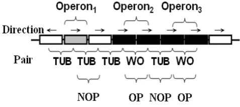
Of the features, the intergenic distance property is the simplest and most widely-used prediction property. It determines whether the distance between gene pairs at the transcription unit borders (TUB pairs) is longer than the distance between gene pairs within an operon (WO pairs). The most important feature is the transcription direction of the genes, which is a straightforward way of identifying the boundaries of certain operons as genes in opposite strands always form part of different operons.
In this study, we propose an effective binary particle swarm optimization (BPSO) for operon prediction. We use the E. coli (NC_000913) dataset, which includes three bacterial genomes [Bacillus subtilis (NC_000964), Pseudomonas aeruginosa PA01 (NC_002516) and S. aureus (NC_002952)] for operon prediction. In a first step, the best possible combination of features is selected based on the concept of feature selection. ROC curves are used to implement the operon prediction. We selected five features commonly used in the literature, namely the intergenic distance, metabolic pathways, COG, gene length ratio and operon length. In a second step, the there most useful feature are employed used through feature selection to evaluate the operons. The experimental results indicate that the proposed method obtains a higher accuracy, sensitivity and specificity on the test data sets when compared to other methods from the literature.
II.METHOD A. Data set
The complete prokaryote genome data used for the tests was obtained from the GenBank database (http://www.ncbi.nlm.nih.gov/). A total of 4488, 4225, 5651 and 2845 genes are contained in the E. coli genome, the B.
An Improved Binary Particle Swarm
Optimization Approach to Operon Prediction
subtilis genome, the P. aeruginosa PA01 genome and the S. aureus genome, respectively. The related genomic information includes the gene name, the gene ID, and the position, strand and product of the gene. The experimental operons of E. coli and B. subtilis were extracted from RegulonDB (http://regulondb.ccg.unam.mx/) [16] and DBTBS (http://dbtbs.hgc.jp/) [17], respectively. The experimental operons of the P. aeruginosa PA01 genome and the S. aureus genome were extracted from the ODB (http://odb.kuicr.kyoto-u.ac.jp/) [11]. RegulonDB and DBTBS collect highly reliable data on experimentally validated operons of the E. coli and the B. subtilis genome [18], respectively. However, experimental operon data of P. aeruginosa PA01, S. aureus isnot listed in any database. Hence, we referred to the literature [19] to extract experimentally validated operons from ODB (Operon DataBase). The metabolic pathway data and the COG data of the genomes were downloaded from KEGG (http://www.genome.ad.jp/kegg/pathway.html) and NCBI (http://www.ncbi.nlm.nih.gov/COG/).
B. Operon pair definition
In order to improve information related to studying drug and protein functions, operons need to be predicted based on an organism’s genomic sequence. The entire genome is searched for adjacent gene pairs, and each gene pair is divided into one of three types: (i) adjacent pair; (ii) OP pair; or (iii) NOP pair. The WO pairs and TUB pairs are defined based on biological experiments; these gene pairs are defined as positive and negative, respectively. If an operon consists of a single gene and the downstream gene of the operon is of unknown status, the adjacent gene is called a TUB pair (Fig. 1). However, if the upstream gene is the last gene of an operon and the downstream gene is of uncertain status, the gene pair cannot be labeled a TUB pair [10]. In addition, the first gene of an operon and the upstream gene is a TUB pair per definition.
C. Operon features
[image:2.595.46.285.669.775.2]In this study, we use feature selection to select the most helpful feature. In a first step, we selected five common features and used Receiver Operating Characteristic (ROC) curves to express the relationship between the sensitivity and specificity value. In a second step, the ROC curves are used to identify where single feature groups have been removed the three most valuable features for operon prediction are selected and the features are individually described below:
Fig. 1. Operon pairs sketch map
a) Intergenic distance
The intergenic distance between two adjacent genes within the same operon tends to be rather short, whereas a distance between two adjacent genes of different operons is relatively long [20]. Much evidence [5, 7, 8, 9, 11] supports the idea that the intergenic distance is the most important feature for operon prediction when it is applied to several genomes.
b) Metabolic pathways
Genes within an operon often share common biological characteristics and occur sequentially or contiguously to fulfill the same or similar functions in the same metabolic pathway [5, 20]. The Kyoto Encyclopedia of Genes and Genomes (KEGG) is one of the best resources for detailed pathway information; this data can be used to predict operons in many organisms.
c) COG gene function
Clusters of orthologous groups (COGs) of proteins [21, 22] are defined by comparing protein sequences encoded in complete genomes. All conserved genes are classified according to their homologous relationships. The COGs are clusters of orthologous groups; individual orthologous proteins typically have the same function, and therefore genes in one operon often are in the same or a similar functional category in COG [14, 23].
d) Gene length ratio
The score of the gene length ratio is determined by the natural logarithm of the length ratio of the upstream gene and the downstream gene [9, 19]. Boundary gene pairs are frequently coupled with small values of the natural logarithm of the length ratio [9], suggesting that the length of the downstream gene in proportion to the upstream gene influences the possibility of co-transcription of two adjacent genes. Therefore, the gene length ratio is one of the important features for operon prediction.
e) Operon length
Genes within one operon are co-transcribed in the same orientation. This characteristic can be used to predict if genes in a genome are clustered into operons. The operon length has been previously used as an operon prediction feature [6, 24]. Bacterial genomes, which typically contain a relatively high number of genes [25], are larger genomes that tend to display less clustering of genes into operons. Therefore, without normalization, the comparison of operon prediction performance between different genomes may be biased
D. Binary particle swarm optimization
and called pbesti. The best value of all the individual pbest
values is called gbest. At each generation, a particle’s position and velocity is updated according to its own pbest and the gbest value of the entire population this behavior is described by Eq. 1 and Eq. 2.
) x gbest ( r c ) x pbest ( r c v w v old id id 2 2 old id id 1 1 old id new id (1) new id oid id new
id x v
x (2)
PSO is a method similar to a genetic algorithm, in which particles are initialized within a random population and search for global optimal solutions at each generation. However, PSO is not suitable for optimization problems in a discrete feature space. Hence, Kennedy and Eberhart developed binary PSO (BPSO) to overcome this problem [27]. The method involves a change in the way velocity is conceptualized. Whereas in a real number space velocity describes a change in position, if might better be thought of as a probability threshold when variables are optimized in a discrete space [27]. If a random number is smaller than the threshold, the variable xidnew is assigned a value of 1,
otherwise it is 0. The function is defined below : ) x exp( 1 1 ) x ( S (3)
Thus the BPSO algorithm can be written as
) x gbest ( r c ) x pbest ( r c v w v old id id 2 2 old id id 1 1 old id new id (4)
If rand() < S(vidnew) then new id
x = 1 else xidnew= 0 (5)
where r1 and r2are random numbers between (0, 1), and c1
and c2 are both set to 2 [28]. Velocities and denote the
velocities of a new particle and an old particle, respectively. The inertia weight w is linearly decreased from 0.9 to 0.4 [28] in the search process in order to optimally balance the global and the local search. The update function is defined below:
min max max min max ) ( w move move move w w
w i
(6)
wmax and wmin are set to 0.9 and 0.4, respectively. movemax
and movei represent the maximum number of iterations and
the current number of iterations, respectively [28].
E. Improved Binary Particle Swarm Optimization
At first particles attract each other the basic PSO algorithm because of the information flow of good solutions between particles. However, Riget et al. define a second phase repulsion [29] by “inverting” the velocity-update formula of the particles:
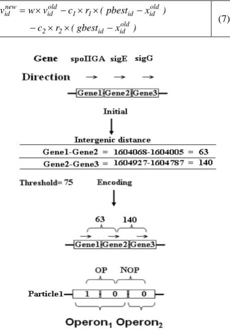
[image:3.595.310.539.50.381.2]) x gbest ( r c ) x pbest ( r c v w v old id id 2 2 old id id 1 1 old id new id (7)
Fig. 2. Initialization and encoding process
In the repulsion phase the individual particle is no longer attracted to, but instead repelled by the best known particle position (gbestid) and its own previous best position
(pbestid).
F. Swarm initialization and code
The initial condition is illustrated in the left part of Fig. 2. Because the first two adjacent genes (Gene1 - Gene2 = 63 bps) have an intergenic distance less than the threshold (75 bps), this pair is considered to be located in the same putative operon. Hence, the first element of the array is 1. Next, the two adjacent genes’ (Gene2-Gene3) distance is 140 bps. Since the threshold is smaller than 140 bps, the two adjacent genes are of different operons, and thus second element of the array is denoted 0. The last gene is always represented as 0 in our encoding, and thus the final encoding of the particle1 is 100.
G.Fitness evaluation
As stated previously, many properties are used to predict operons. In this study, five features are used and described individually in the following section. The pair-scores of the intergenic distance, the metabolic pathway, COG, the gene length ratio and operon length are calculated by the logarithmic likelihood ratio test.
(1) Intergenic distance
We calculate the score of each separated interval in 10 bps bins [30] based on an intergenic distance from -100 bps to 300 bps using the following Eq. 8.
TUB TUB WO WO j i dist TN property N TN property N gene gene / / ln , LL (8)(2) Metabolic pathways
The pathway pair-score is only taken into account when two adjacent genes have the same pathway. Otherwise the pathway pair-score is 0 [19]. Eq. 9 is used to calculate the pathway pair-score.
TUB TUB WO WO j i path TN path N TN path N gene gene / / ln , LL (9)(3) COG gene function
Adjacent genes are often of the same class, so we assume that the gene pair is located in the same operon. The pair-score of the COG gene function is calculated with Eq. 10 based on the first level.
TUB TUB WO WO j i COG TN COG N TN COG N gene gene / / ln , LL (10)
TUB TUB WO WO j i d COG TN COG N TN COG N gene gene / 1 / 1 ln , LL(4) Gene length ratio.
The pair-score of the gene length ratio is calculated as the natural logarithm of the length ratio of upstream genes and downstream genes [9]. It is defined by the following Eq. 11.
j i j i glr length length genegene, ln
LL (11)
(5) Operon length
The operon length is given by the number of genes in an operon [6].The probability P, i.e., the pair-score of the operon length, is calculated by the following Eq. 12.
n
n
P
i1
(12)Finally, the fitness value of a particle is calculated as the sum of the fitness values from all putative operons in the particle and thus given by the following Eq .13.
c i ifitness
fitness
1 (13) where c is the number of operons in the particle.H. Performance evaluation
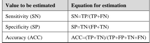
In order to verify the generalization ability of our method, the test of data sets does not contain the E. coli genome because it contains which has genome-specific properties. The predictive performance [9] was evaluated based on the sensitivity and specificity shown in Table 1. In Table 2, the
true positive (TP) and false negative (FN) are the numbers of both correct and incorrect prediction of gene pairs among the WO gene pairs, respectively, whereas the true negative (TN) and the false positive (FP) are the numbers of the correct and incorrect prediction of gene pairs among the TUB gene pairs. The sensitivity, specificity and accuracy are determined based on TP, FN, TN and FP.
Table 1. Evaluation method for operon prediction Value to be estimated Equation for estimation
Sensitivity (SN) SN=TP/(TP+FN)
Specificity (SP) SP=TN/(FP+TN)
Accuracy (ACC) ACC=(TP+TN)/(TP+FP+TN+FN)
Table 2. The positive and negative evaluation True data
Prediction result Positive Negative
Positive TP FP
Negative FN TN
III. RESULTS AND DISCUSSION A. Parameter Settings
The population number was set to 30, the iteration number was 100, c1 and c2 were 2, and Vmax and Vmin were 6 and -6, respectively [26, 27, 28].
[image:4.595.302.552.163.236.2] [image:4.595.41.289.293.362.2]Fig. 3. ROC curves using a single feature.
C.Comparison to other methods
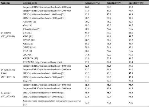
[image:5.595.89.244.52.204.2]An improved BPSO was applied to search for the best putative operon at each generation. The best putative operon identified by the search was then compared to experimentally verified operons. We compared our method with various reported methods, including UNIPOP [2], genetic algorithm (GA) [19], a fuzzy genetic algorithm (FGA) [5], support vector machine (SVM) [7] using both genome-specific and general genomic information [9], VIMSS [14], genome-wide operon prediction in Staphylococcus aureus (S. aureus) [15] and JPOP [8]. As Table 2 shows, the prediction accuracy of the proposed method obtained the highest accuracy value on the B. subtilis (92.5), P. aeruginosaPA01 (93.6), and S. aureus
(95.9) data sets. The proposed method also showed the best performance in terms of prediction sensitivity and specificity on most of the tested bacterial genomes. For P. aeruginosa and S. aureus, our method had the highest sensitivity (93.3) and (95.9), respectively. However, ODB achieved the highest specificity (99.2), but a very low sensitivity (49.9). ODB does not achieve a good balance between sensitivity and specificity as its highs specificity is traded for a low sensitivity. For B. subtilis, P. aeruginosa PA01 and S. aureus, our predictor obtained a higher accuracy and sensitivity compared to the other methods from the literature.
Overall, the proposed method obtained better operon prediction results than the other methods tested.
IV. CONCLUSION
[image:5.595.43.529.236.586.2]In this paper, we propose an improved BPSO method and use the feature selection concept to predict operon. The intergenic distance, metabolic pathway, COG gene functions, gene length ratio, and the operon length of the E. coli genome were employed for feature selection and to design a fitness function. Finally, the method is used to predict operons based on the intergenic distance, metabolic pathway, and gene length ratio, the three best-performing features. Experimental results show that the prediction accuracy, sensitivity and specificity achieved was better than in other methods, and that computation time could be reduced. In the future, we expect to improve our proposed methods by combining other algorithms in order to achieve
Table 3. Accurcy, sensitivity, and specificity of operon prediction on three genomes.
Genome Methodology Accuracy (%) Sensitivity (%) Specificity (%)
B. subtilis (NC_000964)
Improved BPSO (initiation threshold = 600 bps) 92.5 87.8 96.3 Improved BPSO (initiation threshold = 300 bps) 91.9 89.4 93.9
BPSO (initiation threshold = 600 bps) [31] 92.1 93.0 89.9 BPSO (initiation threshold = 300 bps) [31] 90.5 88.7 94.5
UNIPOP [2] 79.2 78.2 82.1
GA [19] 88.3 87.3 89.7
Classification [9] 90.2 N/A N/A
SVM [7] 88.9 90.0 86.0
ODB [11] 63.2 49.9 99.2
DVDA [12] 48.5 31.9 93.2
OFS [32] 68.3 76.5 43.9
VIMSS [14] 78.0 76.4 87.1
FGA [5] 88.2 N/A N/A
JPOP [8] 74.6 72.0 90.0
OPERON [33] 62.9 53.1 89.2
FGENESB (http://www.softberry.com) 77.1 72.1 90.4
P. aeruginosa PA01 (NC_002516)
Improved BPSO (initiation threshold = 600 bps) 93.6 93.3 94.1 Improved BPSO (initiation threshold = 300 bps) 92.2 91.1 94.0 BPSO (initiation threshold = 600 bps) [31] 93.3 93.0 95.1
BPSO (initiation threshold = 300 bps) [31] 91.0 88.5 95.1
GA [19] 81.3 87.0 76.3
S. aureus (NC_002952)
Improved BPSO (initiation threshold = 600 bps) 95.9 95.9 95.9
Improved BPSO (initiation threshold = 300 bps) 93.6 93.1 94.5 BPSO (initiation threshold = 600 bps) [31] 95.9 95.9 95.8 BPSO (initiation threshold = 300 bps) [31] 93.6 92.4 95.8 Genome-wide operon prediction in Staphylococcus aureus
[15] 92.0 N/A N/A
even better results and feature increase the prediction performance.
REFERENCES
[1] De Hoon, M., S. Imoto, K. Kobayashi, N. Ogasawara, and S. Miyano. 2004. Predicting the operon structure of Bacillus subtilis using operon length, intergene distance, and gene expression information. Citeseer. pp. 276–287.
[2] Li,G., Che,D. and Xu,Y. (2009) A universal operon predictor for prokaryotic genomes. J Bioinform Comput Biol., 7, 19–38.
[3] Moreno-Hagelsieb G, Collado-Vides J. A powerful nonhomology method for the prediction of operons in prokaryotes. Bioinformatics 2002;18:S329–36.
[4] De Hoon MJ, Imoto S, Kobayashi K, et al. Predicting the operon structure of Bacillus subtilis using operon length, intergene distance, and gene expression information. Pac Symp Biocomput 2004;276–87. [5] Jacob E, Sasikumar R, Nair KN. A fuzzy guided genetic algorithm for
operon prediction. Bioinformatics 2005;21: 1403–7
[6] Bockhorst J, Craven M, Page D, et al. A Bayesian network approach to operon prediction. Bioinformatics 2003;19:1227–35.
[7] Zhang GQ, Cao ZW, Luo QM, et al. Operon prediction based on SVM. Comput Biol Chem 2006;30:233–40.
[8] Chen X, Su Z, Dam P, et al. Operon prediction by comparative genomics: an application to the Synechococcus sp. WH8102 genome. Nucleic Acids Res 2004;32:2147–57.
[9] Dam P, Olman V, Harris K et al. Operon prediction using both genome-specific and general genomic information, Nucleic Acids Res. 2007;35:288-298.
[10] Sabatti C, Rohlin L, Oh MK et al. Co-expression pattern from DNA microarray experiments as a tool for operon prediction, Nucleic Acids Res. 2002;30:2886-2893.
[11] Okuda S, Katayama T, Kawashima S et al. ODB: a database of operons accumulating known operons across multiple genomes, Nucleic Acids Res. 2006;34:D358-D362.
[12] Edwards,M.T., Rison,S.C., Stoker,N.G. and Wernisch,L. (2005) A universally applicable method of operon map prediction on minimally annotated genomes using conserved genomic context. Nucleic Acids Res., 33, 3253–3262.
[13] Chen,X., Su,Z., Dam,P., Palenik,B., Xu,Y. and Jiang,T. (2004) Operon prediction by comparative genomics: an application to the Synechococcus sp. WH8102 genome. Nucleic Acids Res., 32, 2147–2157.
[14] Price,M.N., Huang,K.H., Alm,E.J. and Arkin,A.P. (2005) A novel method for accurate operon predictions in all sequenced prokaryotes. Nucleic Acids Res., 33, 880–892.
[15] Wang,L., Trawick,J.D., Yamamoto,R. and Zamudio,C. (2004) Genome-wide operon prediction in Staphylococcus aureus. Nucleic Acids Res., 32, 3689–3702.
[16] Pertea, M., Yanbule, K., Smedinghoff, M., Salzberg, S.L., 2008. OperonDB: a comprehensive database of predicted operons in microbial genomes. Nucleic Acids Res. 37, D479-482.
[17] Sierro, N., Makita, Y., De Hoon, M., Nakai, K., 2008. DBTBS: a database of transcriptional regulation in Bacillus subtilis containing upstream intergenic conservation information. Nucleic Acids Res. 36, D93-D96.
[18] Mao, F., Dam, P., Chou, J., OlmanL, V., XU, Y., 2009. DOOR: a database for prokaryotic operons. Nucleic Acids Res. 37, D459-463. [19] Wang, S., Wang, Y., Du, W., Sun, F., Wang, X., Zhou, C., Liang, Y.,
2007. A multi-approaches-guided genetic algorithm with application to operon prediction. Artif Intell Med 41, 151-159.
[20] Salgado H, Moreno-Hagelsieb G, Smith TF et al. Operons in Escherichia coli: genomic analyses and predictions, Proc. Natl Acad. Sci. 2000;97:6652-6657.
[21] Tatusov R, Koonin E, Lipman D. A genomic perspective on protein families, Science 1997;278:631.
[22] Tatusov R, Fedorova N, Jackson J et al. The COG database: an updated version includes eukaryotes, BMC Bioinformatics 2003;4:41. [23] Chen X, Su Z, Xu Y et al. Computational prediction of operons in
Synechococcus sp. WH8102, Genome Inform 2004;15:211-222. [24] Craven M, Page D, Shavlik J et al. A probabilistic learning approach
to whole-genome operon prediction, Proc Int Conf Intell Syst Mol Biol 2000;8:116-127.
[25] Cherry JL. Genome size and operon content, J Theor Biol 2003;221:401-410.
[26] Kennedy,J. and Eberhart,R. (1995) Particle swarm optimization. Proceedings of the IEEE International Conference on Neural Networks, Vol. 4, pp. 1942–1948.
[27] Kennedy,J. and Eberhart,R. (1997) A discrete binary version of the particle swarm algorithm. Proceedings of the IEEE International Conference on Systems, Man, and Cybernetics, Vol. 5, pp. 4104–4108.
[28] Poli, R., J. Kennedy, and T. Blackwell. “Particle swarm optimization”. Swarm Intelligence, vol.1, pp. 33-57. 2007
[29] Riget, J., and J. Vesterstrom. 2002. A diversity-guided particle swarm optimizer-the ARPSO. Dept. Comput. Sci., Univ. of Aarhus, Aarhus, Denmark, Tech. Rep 2:2002.
[30] Romero, P.R. and Karp, P.D. (2004) Using functional and organizational information to improve genome-wide computational prediction of transcription units on pathway-genome databases. Bioinformatics, 20, 709-717.
[31] Chuang L, Tsai J, Yang C. Binary particle swarm optimization for operon prediction, Nucleic acids research 2010;38:e128.
[32] Westover, B.P., Buhler, J.D., Sonnenburg, J.L. and Gordon, J.I. (2005) Operon prediction without a training set. Bioinformatics, 21, 880-888.