Universal Dependency Parsing from Scratch

Proceedings of the CoNLL 2018 Shared Task: Multilingual Parsing from Raw Text to Universal Dependencies, pages 160–170 Brussels, Belgium, October 31 – November 1, 2018. c2018 Association for Computational Linguistics

160

Universal Dependency Parsing from Scratch

Peng Qi,* Timothy Dozat,* Yuhao Zhang,* Christopher D. Manning Stanford University

Stanford, CA 94305

{pengqi, tdozat, yuhaozhang, manning}@stanford.edu

Abstract

This paper describes Stanford’s system at the CoNLL 2018 UD Shared Task. We introduce a complete neural pipeline sys-tem that takes raw text as input, and per-forms all tasks required by the shared task, ranging from tokenization and sentence segmentation, to POS tagging and depen-dency parsing. Our single system sub-mission achieved very competitive perfor-mance on big treebanks. Moreover, after fixing an unfortunate bug, our corrected system would have placed the 2nd, 1st, and 3rdon the official evaluation metrics LAS, MLAS, and BLEX, and would have out-performed all submission systems on low-resource treebank categories on all metrics by a large margin. We further show the ef-fectiveness of different model components through extensive ablation studies.

1 Introduction

Dependency parsing is an important component in various natural langauge processing (NLP) sys-tems for semantic role labeling (Marcheggiani and Titov, 2017), relation extraction (Zhang et al., 2018), and machine translation (Chen et al.,2017). However, most research has treated dependency parsing in isolation, and largely ignored upstream NLP components that prepare relevant data for the parser, e.g., tokenizers and lemmatizers (Zeman et al., 2017). In reality, however, these upstream systems are still far from perfect.

To this end, in our submission to the CoNLL 2018 UD Shared Task, we built a raw-text-to-CoNLL-U pipeline system that performs all tasks required by the Shared Task (Zeman et al.,

∗

These authors contributed roughly equally.

2018).1 Harnessing the power of neural sys-tems, this pipeline achieves competitive perfor-mance in each of the inter-linked stages: tok-enization, sentence and word segmentation, part-of-speech (POS)/morphological features (UFeats) tagging, lemmatization, and finally, dependency parsing. Our main contributions include:

• New methods for combining symbolic statis-tical knowledge with flexible, powerful neu-ral systems to improve robustness;

• A biaffine classifier for joint POS/UFeats pre-diction that improves prepre-diction consistency;

• A lemmatizer enhanced with aneditclassifier that improves the robustness of a sequence-to-sequence model on rare sequences; and

• Extensions to our parser from (Dozat et al., 2017) to model linearization.

Our system achieves competitive performance on big treebanks. After fixing an unfortunate bug, the corrected system would have placed the 2nd, 1st, and 3rdon the official evaluation metrics LAS, MLAS, and BLEX, and would have outperformed all submission systems on low-resource treebank categories on all metrics by a large margin. We perform extensive ablation studies to demonstrate the effectiveness of our novel methods, and high-light future directions to improve the system.2

2 System Description

In this section, we present detailed descriptions for each component of our neural pipeline system, namely the tokenizer, the POS/UFeats tagger, the lemmatizer, and finally the dependency parser.

1_{We chose to develop a pipeline system mainly because it}

allows easier parallel development and faster model tuning in a shared task context.

2_{To facilitate future research, we make our}

implementa-tion public at:https://github.com/stanfordnlp/

2.1 Tokenizer

To prepare sentences in the form of a list of words for downstream processing, the tokenizer compo-nent reads raw text and outputs sentences in the CoNLL-U format. This is achieved with two sub-systems: one for joint tokenization and sentence segmentation, and the other for splitting multi-word tokens into syntactic multi-words.

Tokenization and sentence segmentation. We

treat joint tokenization and sentence segmentation as a unit-level sequence tagging problem. For most languages, aunit of text is a single charac-ter; however, in Vietnamese orthography, the most natural units of text are singlesyllables.3 We as-sign one out of five tags to each of these units: end of token (EOT), end of sentence (EOS), multi-word

token (MWT), multi-word end of sentence (MWS), and other (OTHER). We use bidirectional LSTMs (BiLSTMs) as the base model to make unit-level predictions. At each unit, the model predicts hier-archically: it first decides whether a given unit is at the end of a token with a scores(tok), then clas-sifies token endings into finer-grained categories with two independent binary classifiers: one for sentence endings(sent), and one for MWTs(MWT). Since sentence boundaries and MWTs usually require a larger context to determine (e.g., periods following abbreviations or the ambiguous word “des” in French), we incorporate token-level infor-mation into a two-layer BiLSTM as follows (see also Figure1). The first layer BiLSTM operates directly on raw units, and makes an initial predic-tion over the categories. To help capture local unit patterns more easily, we also combine the first-layer BiLSTM with 1-D convolutional networks, by using a one hidden layer convolutional network (CNN) with ReLU nolinearity at its first layer, giv-ing an effect a little like a residual connection (He et al., 2016). The output of the CNN is simply added to the concatenated hidden states of the Bi-LSTM for downstream computation:

hRNN₁ = [−h→1,

←−

h1] =BiLSTM1(x), (1)

hCNN₁ =CNN(x), (2)

h1 =hRNN1 +hCNN1 , (3)

[s(₁tok),s₁(sent),s(MWT)₁ ] =W1h1, (4)

where x is the input character representations,

3_{In this case, we define a syllable as a consecutive run}

of alphabetic characters, numbers, or individual symbols, to-gether with any leading white spaces before them.

BiLSTM1

Step t

Input Unitt 1-D CNN

!_",$(&'()) !_",$(+,-) _! ",$()./)

!_0,$(&'()) !_0,$(+,-) _! 0,$()./) !_$(&'()) !_$(+,-) _!

$()./)

σ +

+

+

Input First layer First layer prediction & gating Second layer Final prediction

Second layer prediction

BiLSTM1

Step t

Figure 1: Illustration of the tokenizer/sentence segmenter model. Components in blue represent the gating mechanism between the two layers.

andW1 contains the weights and biases for a lin-ear classifier.4 For each unit, we concatenate its trainable embedding with a four-dimensional bi-nary feature vector as input, each dimension cor-responding to one of the following feature func-tions: (1) does the unit start with whitespace; (2) does it start with a capitalized letter; (3) is the unit fully capitalized; and (4) is it purely numerical.

To incorporate token-level information at the second layer, we use a gating mechanism to sup-press representations at non-token boundaries be-fore propagating hidden states upward:

g1=h1σ(s(1tok)) (5)

h2= [

−→

h2,

←−

h2] =BiLSTM2(g1), (6)

[s(₂tok),s₂(sent),s(MWT)₂ ] =W2h2, (7)

where is an element-wise product broadcast over all dimensions of h1 for each unit. This can be viewed as a simpler alternative to multi-resolution RNNs (Serban et al., 2017), where the first-layer BiLSTM operates at the unit level, and the second layer operates at the token level. Unlike multi-resolution RNNs, this formulation is end-to-end differentiable, and can more easily leverage efficient off-the-shelf RNN implementations.

To combine predictions from both layers of the BiLSTM, we simply sum the scores to obtain

s(X)=s(X)₁ +s₂(X), whereX∈ {tok, sent,MWT}. The final probability over the tags is then

pEOT =p+−− pEOS =p++−, (8)

pMWT=p+−+ pMWS=p+++, (9)

wherep±±± =σ(±s(tok))σ(±s(sent))σ(±s(MWT)),

andσ(·)is the logistic sigmoid function.pOTHERis simplyσ(−s(tok)_{). The model is trained to}

mini-mize the standard cross entropy loss.

Multi-word Token Expansion. The tokenizer/

sentence segmenter produces a collection of sen-tences, each being a list of tokens, some of which are labeled as multi-word tokens (MWTs). We must expand these MWTs into the underlying syn-tactic words they correspond to (e.g., “im” to “in dem” in German), in order for downstream sys-tems to process them properly. To achieve this, we take a hybrid approach to combine symbolic statis-tical knowledge with the power of neural systems. The symbolic statistical side is a frequency lex-icon. Many languages, like German, have only a handful of rules for expanding a few MWTs. We leverage this information by simply counting the number of times a MWT is expanded into differ-ent sequences of words in the training set, and re-taining the most frequent expansion in a dictionary to use at test time. When building this dictionary, we lowercase all words in the expansions to im-prove robustness. However, this approach would fail for languages with rich clitics, a large set of unique MWTs, and/or complex rules for MWT ex-pansion, such as Arabic and Hebrew. We capture this by introducing a powerful neural system.

Specifically, we train a sequence-to-sequence model using a BiLSTM encoder with an attention mechanism (Bahdanau et al.,2015) in the form of a multi-layer perceptron (MLP). Formally, the in-put multi-word token is represented by a sequence of charactersx1, . . . , xI, and the output syntactic words are represented similarly as a sequence of characters y1, . . . , yJ, where the words are sep-arated by space characters. Inputs to the RNNs are encoded by a shared matrix of character em-beddingsE. Once the encoder hidden stateshenc

are obtained with a single-layer BiLSTM, each de-coder step is unrolled as follows:

hdec_j =LSTMdec(Eyj−1,h dec

j−1), (10)

αij ∝exp(u>αtanh(Wα[hdecj ,henci ])), (11)

cj =

X

i

αijhenci , (12)

P(yj =w|y<j)∝u>wtanh(W[hdecj ,cj]). (13)

Here,w is a character index in the output vocab-ulary,y0a special start-of-sequence symbol in the vocabulary, andhdec₀ the concatenation of the last hidden states of each direction of the encoder.

To bring the symbolic and neural systems to-gether, we train them separately and use the fol-lowing protocol during evaluation: for each MWT, we first look it up in the dictionary, and return the expansion recorded there if one can be found. If this fails, we retry by lowercasing the incoming token. If that fails again, we resort to the neural system to predict the final expansion. This allows us to not only account for languages with flexi-ble MWTs patterns (Arabic and Hebrew), but also leverage the training set statistics to cover both languages with simpler MWT rules, and MWTs in the flexible languages seen in the training set without fail. This results in a high-performance, robust system for multi-word token expansion.

2.2 POS/UFeats Tagger

Our tagger follows closely that of (Dozat et al., 2017), with a few extensions. As in that work, the core of the tagger is a highway BiLSTM ( Sri-vastava et al.,2015) with inputs coming from the concatenation of three sources: (1) a pretrained word embedding, from the word2vec embeddings provided with the task when available (Mikolov et al., 2013), and from fastText embeddings oth-erwise (Bojanowski et al., 2017); (2) a trainable frequent word embedding, for all words that oc-curred at least seven times in the training set; and (3) a character-level embedding, generated from a unidirectional LSTM over characters in each word. UPOS is predicted by first transforming each word’s BiLSTM state with a fully-connected (FC) layer, then applying an affine classifier:

hi =BiLSTM(_itag)(x1, . . . ,xn), (14)

v(_iu)=FC(u)(hi), (15)

P y_ik(u)|X

=softmaxk W(u)v (u) i

. (16)

To predict XPOS, we similarly start with trans-forming the BiLSTM states with an FC layer. In order to further ensure consistency between the different tagsets (e.g., to avoid aVERBUPOS with an NNXPOS), we use abiaffineclassifier, condi-tioned on a word’s XPOS state as well as an em-bedding for its gold (at training time) or predicted (at inference time) UPOS tagy(_i∗u):

v(_ix)=FC(x)(hi), (17)

s(_ix)= [E(u)

y_i(u)∗

,1]>U(x)[v(_ix),1], (18)

P y_ik(x)|y_i(_∗u), X=softmaxk s (x) i

UFeats is predicted analogously with separate pa-rameters for each individual UFeat tag. The tagger is also trained to minimize the cross entropy loss.

Some languages have composite XPOS tags, yielding a very large XPOS tag space (e.g., Arabic and Czech). For these languages, the biaffine clas-sifier requires a prohibitively large weight tensor

U(x). For languages that use XPOS tagsets with a fixed number of characters, we classify each char-acter of the XPOS tag in the same way we clas-sify each UFeat. For the rest, instead of taking the biaffine approach, we simply share the FC layer between all three affine classifiers, hoping that the learned features for one will be used by another.

2.3 Lemmatizer

For the lemmatizer, we take a very similar ap-proach to that of the multi-word token expansion component introduced in Section2.1with two key distinctions customized to lemmatization.

First, we build two dictionaries from the train-ing set, one from a (word, UPOS) pair to the lemma, and the other from the word itself to the lemma. During evaluation, the predicted UPOS is used. When the UPOS-augmented dictionary fails, we fall back to the word-only dictionary before resorting to the neural system. In look-ing up both dictionaries, the word is never lower-cased, because case information is more relevant in lemmatization than in MWT expansion.

Second, we enhance the neural system with an editclassifier that shortcuts the prediction process to accommodate rare, long words, on which the decoder is more likely to flounder. The concate-nated encoder final states are put through an FC layer with ReLU nonlinearity and fed into a 3-way classifier, which predicts whether the lemma is (1) exactly identical to the word (e.g., URLs and emails), (2) the lowercased version of the word (e.g., capitalized rare words in English that are not proper nouns), or (3) in need of the sequence-to-sequence model to make more complex edits to the character sequence. During training time, we assign the labels to each word-lemma pair greed-ily in the order of identical, lowercase, and se-quence decoder, and train the classifier jointly with the sequence-to-sequence lemmatizer. At evalua-tion time, predicevalua-tions are made sequentially, i.e., the classifier first determines whether any shortcut can be taken, before the sequence decoder model is used if needed.

2.4 Dependency Parser

The dependency parser also follows that of (Dozat et al.,2017) with a few augmentations. The high-way BiLSTM takes as input pretrained word em-beddings, frequent word and lemma emem-beddings, character-level word embeddings, summed XPOS and UPOS embeddings, and summed UFeats em-beddings. In (Dozat et al.,2017), unlabeled attach-ments are predicted by scoring each wordiand its potential heads with a biaffine transformation

ht=BiLSTM(tparse)(x1, . . . ,xn), (20)

v_i(ed),v(_jeh)=FC(ed)(hi),FC(eh)(hj), (21)

s(_ije)= [v(_jeh),1]>U(e)[v_i(ed),1], (22)

=Deep-Biaff(e)(hi,hj), (23)

P y(_ije)|X

=softmaxj s(ie)

, (24)

where v(ed)_i is word i’s edge-dependent repre-sentation and v(eh)_i its edge-head representation. This approach, however, does not explicitly take into consideration relative locations of heads and dependents during prediction; instead, such pre-dictive location information must be implicitly learned by the BiLSTM. Ideally, we would like the model to explicitly condition on(i−j), namely the dependentiand its potential headj’s location relative to each other, in modelingp(yij).5

Here, we motivate one way to build this into the model. First we factorize the relative loca-tion of wordi and head j into their linear order and thedistancebetween them,i.e.,P(yij|sgn(i−

j),abs(i−j)), where sgn(·) is the sign function. Applying Bayes’ rule and assuming conditional independence, we arrive at the following

P(yij|sgn(i−j),abs(i−j))∝ (25)

P(yij)P(sgn(i−j)|yij)P(abs(i−j)|yij).

In a language where heads always follow their de-pendents, P(sgn(i−j) = 1|yij) would be ex-tremely low, heavily penalizing rightward attach-ments. Similarly, in a language where dependen-cies are always short,P(abs(i−j)0|yij)would be extremely low, penalizing longer edges.

P(yij) can remain the same as computed in Eq. (24).P(sgn(i−j)|y_ij)can be computed sim-ilarly with a deep biaffine scorer (cf. Eqs. (20)– (23)) over the recurrent states. This results in the score ofjprecedingi; flipping the sign wherever

iprecedesjturns this into the log odds of the

served linearization. Applying the sigmoid func-tion then turns it into a probability:

s(_ijl)=Deep-Biaff(l)(hi,hj), (26)

s0_ij(l)=sgn(i−j)s(_ijl), (27)

P(sgn(i−j)|y_ij) =σ s0_ij(l)

. (28)

This can be effortlessly incorporated into the edge score by adding in the log of this probability

−log(1 + exp(−s0_ij(l))). Error is not backpropa-gated to this submodule through the final attach-ment loss; instead, it is trained with its own cross entropy, with error only computed on gold edges. This ensures that the model learns the conditional probability given a true edge, rather than just learning to predict the linear order of two words.

ForP(abs(i−j)|yij), we use another deep bi-affine scorer to generate a distance score. Dis-tances are always no less than 1, so we apply

1 +softplus to predict the distance betweeniand

jwhen there’s an edge between them:

s(_ijd)=Deep-Biaff(d)(hi,hj), (29)

s0_ij(d)= 1 +softplus s(_ijd)

. (30)

where softplus(x) = log(1 + exp(x)). The dis-tribution of edge lengths in the treebanks roughly follows a Zipfian distribution, to which the Cauchy distribution is closely related, only the latter is more stable for values at or near zero. Thus, rather than modeling the probability of an arc’s length, we can use the Cauchy distribution to model the probability of an arc’s error in predicted length, namely how likely it is for the predicted distance and the true distance to have a difference ofδ(_ijd):

Zipf(k;α, β)∝(kα/β)−1, (31)

Cauchy(x;γ)∝(1 +x2/γ)−1 (32)

δ_ij(d)=abs(i−j)−s0_ij(d), (33)

P(abs(i−j)|yij)∝(1 +δ_ij2(d)/2)−1. (34)

When the difference δ_ij(d) is small or zero, there will be effectively no penalty; but when the model expects a significantly longer or shorter arc than the observed distance between i andj, it is dis-couraged from assigning an edge between them. As with the linear order probability, the log of the distance probability is added to the edge score, and trained with its own cross-entropy on gold edges.6

6_{Note that the penalty assigned to the edge score in this}

way is proportional tolnδ_ij(d)for highδ_ij(d); using a Gamma

At inference time, the Chu-Liu/Edmonds algo-rithm (Chu and Liu,1965;Edmonds,1967) is used to ensure a maximum spanning tree. Dependency relations are assigned to gold (at training time) or predicted (at inference time) edges y_i(_∗e) using another deep biaffine classifier, following (Dozat et al.,2017) with no augmentations:

s(_ir)=Deep-Biaff(r) hi,h_y(e)

i∗

, (35)

P y(_ikr)|y_i(_∗e)

=softmaxk s(_ir). (36)

3 Training Details

Except where otherwise stated, our system is a pipeline: given a document of raw text, the to-kenizer/sentence segmenter/MWT expander first splits it into sentences of syntactic words; the tag-ger then assigns UPOS, XPOS and UFeat tags to each word; the lemmatizer takes the predicted word and UPOS tag and outputs a lemma; finally, the parser takes all annotations as input and pre-dicts the head and dependency label for each word. All components are trained with early stopping on the dev set when applicable. When a dev set is unavailable, we split the training set into an approximately 7-to-1 split for training and de-velopment. All components (except the depen-dency parser) are trained and evaluated on the de-velopment set assuming all related components had oracle implementations. This means the to-kenizer/sentence segmenter assumes all correctly predicted MWTs will be correctly expanded, the MWT expander assumes gold word segmentation, and all downstream tasks assume gold word seg-mentation, along with gold annotations of all pre-requisite tasks. The dependency parser is trained with predicted tags and morphological features from the POS/UFeats tagger.

Treebanks without training data. For

tree-banks without training data, we adopt a heuristic approach for finding replacements. Where a larger treebank in the same language is available (i.e., all PUD treebanks and Japanese-Modern), we used the models from the largest treebank available in that language. Where treebanks in related lan-guages are available (as determined by language families from Wikipedia), we use models from the largest treebank in that related language. We

ended up choosing the models from English-EWT for Naija (an English-based pidgin), Irish-IDT for Breton (both are Celtic), and Norwegian-Nynorsk for Faroese (both are West Scandinavian). For Thai, since it uses a different script from all other languages, we use UDPipe 1.2 for all components.

Hyperparameters. The tokenizer/sentence

seg-menter uses BiLSTMs with 64d hidden states in each direction and takes 32d character em-beddings as input. During training, we employ dropout to the input embeddings and hidden states at each layer with p = .33. We also randomly replace the input unit with a special<UNK> unit withp=.33, which would be used in place of any unseen input at test time. We add noise to the gat-ing mechanism in Eq. (6) by randomly setting the gates to 1 withp=.02and setting its temperature to 2 to make the model more robust to tokeniza-tion errors at test time. Optimizatokeniza-tion is performed with Adam (Kingma and Ba, 2015) with an ini-tial learning rate of .002 for up to 20,000 steps, and whenever dev performance deteriorates, as is evaluated every 200 steps after the 2,000th step, the learning rate is multiplied by .999. For the convolutional component we use filter sizes of 1 and 9, and for each filter size we use 64 channels (same as one direction in the BiLSTM). The con-volutional outputs are concatenated in the hidden layer, before an affine transform is applied to serve as a residual connection for the BiLSTM. For the MWT expander, we use BiLSTMs with 256d hid-den states in each direction as the encoder, a 512d LSTM decoder, 64d character embeddings as in-put, and dropout rate p = .5 for the inputs and hidden states. Models are trained up to 100 epochs with the standard Adam hyperparameters, and the learning rate is annealed similarly every epoch af-ter the 15th epoch by a factor of0.9. Beam search of beam size 8 is employed in evaluation.

The lemmatizer uses BiLSTMs with 100d hid-den states in each direction of the encoder, 50d character embeddings as input, and dropout rate

p = .5 for the inputs and hidden states. The de-coder is an LSTM with 200d hidden states. During training we jointly minimize (with equal weights) the cross-entropy loss of the edit classifier and the negative log-likelihood loss of the seq2seq lem-matizer. Models are trained up to 60 epochs with standard Adam hyperparameters.

The tagger and parser share most of their hy-perparameters. We use 75d uncased frequent

word and lemma embeddings, and 50d POS tag and UFeat embeddings. Pretrained embeddings and character-based word representations are both transformed to be 125d. During training, all em-beddings are randomly replaced with a<drop>

symbol withp = .33. We use 2-layer 200d BiL-STMs for the tagger and 3-layer 400d BiLBiL-STMs for the parser. We employ dropout in all feed-forward connections with p = .5 and all recur-rent connections (Gal and Ghahramani,2016) with

p = .25 (exceptp = .5 in the tagger BiLSTM). All classifiers use 400d FC layers (except 100d for UFeats) with the ReLU nonlinearity. We train the systems with Adam (α = .003, β1 = .9,

β2 = .95) until dev accuracy decreases, at which point we switch to AMSGrad (Reddi et al.,2018) until 3,000 steps pass with no dev accuracy in-creases.

4 Results

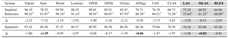
The main results are shown in Table1. As can be seen from the table, our system achieves competi-tive performance on nearly all of the metrics when macro-averaged over all treebanks. Moreover, it achieves the top performance on several metrics when evaluated only on big treebanks, showing that our systems can effectively leverage statisti-cal patterns in the data. Where it is not the top per-forming system, our system also achieved compet-itive results on each of the metrics on these tree-banks. This is encouraging considering that our system is comprised of single-system components, whereas some of the best performing teams used ensembles (e.g., HIT-SCIR (Che et al.,2018)).

When taking a closer look, we find that our UFeats classifier is very accurate on these tree-banks as well. Not only did it achieve the top performance on UFeats F1, but also it helped the parser achieve top MLAS as well on big treebanks, even when the parser is not the best-performing as evaluated by other metrics. We also note the contribution from our consistency modeling in the POS tagger/UFeats classifier: in both settings the individual metrics (UPOS, XPOS, and UFeats) achieve a lower advantage margin over the refer-ence systems when compared to the AllTags met-ric, showing that these reference systems, though sometimes more accurate on each individual task, are not as consistent as our system overall.

(a) Results on all treebanks

System Tokens Sent Words Lemmas UPOS XPOS UFeats AllTags UAS CLAS LAS MLAS BLEX

Stanford 96.19 76.55 95.99 88.32 89.01 85.51 85.47 79.71 76.78 68.73 72.29 60.92 64.04 Reference 98.42† 83.87† 98.18‡ 91.24? _90.91‡ _86.67∗ _87.59‡ _80.30∗ _80.51† _72.36† _75.84† _61.25∗ _66.09?

∆ –2.23 –7.32 –2.19 –2.92 –1.90 –1.16 –2.12 –0.59 –3.73 –3.63 –3.55 –0.33 –2.05

Stanford+ 97.42 85.46 97.23 89.17 89.95 86.50 86.20 80.36 79.04 70.39 74.16 62.08 65.28

∆ –1.00 +1.59 –0.95 –2.07 –0.96 –0.17 –1.39 +0.06 –1.47 –1.97 –1.68 +0.83 –0.81

(b) Results on big treebanks only

System Tokens Sent Words Lemmas UPOS XPOS UFeats AllTags UAS CLAS LAS MLAS BLEX

Stanford 99.43 89.52 99.21 95.25 95.93 94.95 94.14 91.50 86.56 79.60 83.03 72.67 75.46 Reference 99.51† 87.73† 99.16† 96.08? 96.23† 95.16† 94.11∗ 91.45∗ 87.61† 81.29† 84.37† 71.71∗ 75.83?

∆ –0.08 +1.79 +0.05 –0.83 –0.30 –0.21 +0.03 +0.05 –1.05 –1.69 –1.34 +0.96 –0.37

Table 1: Evaluation results (F1) on the test set, on all treebanks and big treebanks only. For each set of results on all metrics, we compare it against results from reference systems. A reference system is the top performing system on that metric if we are not top, or the second-best performing system on that metric. Reference systems are identified by superscripts (†: HIT-SCIR, ‡: Uppsala, ?: TurkuNLP,∗: UDPipe Future). Shaded columns in the table indicate the three official evaluation metrics. “Stanford+” is our system after a bugfix evaluated unofficially; for more details please see the main text.

Treebanks System LAS MLAS BLEX

Small Stanford+ 83.90 72.75 77.30

Reference 69.53† 49.24‡ 54.89‡

Low-Res Stanford+ 63.20 51.64 53.58

Reference 27.89? _6.13? _13.98?

PUD Stanford+ 82.25 74.20 74.37

Reference 74.20† 58.75∗ 63.25•

Table 2: Evaluation results (F1) on low-resource treebank test sets. Reference systems are identi-fied by symbol superscripts (†: HIT-SCIR,‡: ICS PAS,?: CUNI x-ling,∗: Stanford,•: TurkuNLP).

segmentation. After inspecting the results on smaller treebanks and double-checking our imple-mentation, we noticed issues with how we pro-cessed data in the tokenizer that negatively im-pacted generalization on these treebanks.7 This is devastating for these treebanks, as all downstream components process words at the sentence level.

We fixed this issue, and trained new tokenizers with all hyperparameters identical to our system at submission. We further built an unofficial evalua-tion pipeline, which we verified achieves the same evaluation results as the official system, and

eval-7

Specifically, our tokenizer was originally designed to be aware of newlines (\n) in double newline-separated para-graphs, but we accidentally prepared training and dev sets for low resource treebanks by putting each sentence on its own line in the text file. This resulted in the sentence segmenter overfitting to relying on newlines. In later experiments, we replaced all in-paragraph whitespaces with space characters.

uated our entire pipeline byonlyreplacing the to-kenizer. As is shown in Table 1, the resulting system (Stanford+) is much more accurate over-all, and we would have ranked 2nd, 1st, and 3rdon the official evaluation metrics LAS, MLAS, and BLEX, respectively.8 On big treebanks, all met-rics changed within only 0.02% F1 and are thus not included. On small treebanks, however, this effect is more pronounced: as is shown in Table 2, our corrected system outperforms all submis-sion systems on all official evaluation metrics on all low-resource treebanks by a large margin.

5 Analysis

In this section, we perform ablation studies on the new approaches we proposed for each component, and the contribution of each component to the fi-nal pipeline. For each component, we assume ac-cess to an oracle for all other components in the analysis, and show their efficacy on the dev sets.9 For the ablations on the pipeline, we report macro-averaged F1on the test set.

8_{We note that the only system that is more accurate than}

ours on LAS is HIT’s ensemble system, and we achieve very close performance to their system on MLAS (only 0.05% F1 lower, which is likely within the statistical variation reported in the official evaluation).

9

System Tokens Sentences Words

Stanford+ 99.46 91.33 99.27

−gating 99.47 91.34 99.27

−conv 99.45 91.03 98.67

−seq2seq – – 98.97

−dropout 99.22∗ 88.78∗∗∗ 98.98∗

Table 3: Ablation results for the tokenizer. All metrics in the table are macro-averaged dev F1.

101 ₁₀2 ₁₀3 ₁₀4

0 5 10

Arabic-PADT

Czech-PDT

Hebrew-HTB

Italian-PoSTWITATurkish-IMST

#MWTs in Training

∆

W

ords

F1

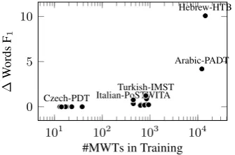
Figure 2: Effect of the seq2seq component for MWT expansion in the tokenizer.

Tokenizer. We perform ablation studies on the

less standard components in the tokenizer, namely the gating mechanism in Eq. (6) (gating), the con-volutional residual connections (conv), and the seq2seq model in the MWT expander (seq2seq), on all 61 big treebanks. As can be seen in Ta-ble 3, all but the gating mechanism make no-ticeable differences in macro F1. When taking a closer look, we find that both gating andconv show a mixed contribution to each treebank, and we could have improved overall performance fur-ther through treebank-level component selection. One surprising discovery is thatconvgreatly helps identify MWTs in Hebrew (+34.89 Words F1) and sentence breaks in Ancient Greek-PROIEL (+18.77 Sents F1). In the case of seq2seq, al-though the overall macro difference is small, it helps with the word segmentation performance on all treebanks where it makes any meaningful difference, most notably +10.08 on Hebrew and

+4.19on Arabic in Words F1 (see also Figure2). Finally, we note that dropout plays an important role in safeguarding the tokenizer from overfitting.

POS/UFeats Tagger. The main novelty in our

tagger is the explicit conditioning of XPOS and UFeats predictions on the UPOS prediction. We compare this against a tagger that simply shares the hidden features between the UPOS, XPOS, and UFeats classifiers. Since we used full-rank tensors in the biaffine classifier, treebanks with

System UPOS XPOS UFeats AllTags PMI

Stanford 96.50 95.87 95.01 92.52 .0514

−biaff 96.47 95.71∗ 94.13∗∗∗ 91.32∗∗∗ .0497∗

Table 4: Ablation results for the tagger. All metrics are macro-averaged dev F1, except PMI, which is explained in detail in the main text.

System Big Small LowRes All

Stanford 96.56 91.72∗ 69.21 94.22

−edit & seq2seq 89.97∗∗∗ 82.68∗∗∗ 63.50∗∗ 87.45∗∗∗

−edit 96.48∗ 91.80 68.30 94.10

−dictionaries 95.37∗∗∗ 90.43∗∗∗ 66.02∗ 92.89∗∗∗

Table 5: Ablation results for the lemmatizer, split by different groups of treebanks. All metrics in the table are macro-averaged dev F1.

large, composite XPOS tagsets would incur pro-hibitive memory requirements. We therefore ex-clude treebanks that either have more than 250 XPOS tags or don’t use them, leaving 36 treebanks for this analysis. We also measure consistency be-tween tags by their pointwise mutual information

PMI= log

pc(AllTags)

pc(UPOS)pc(XPOS)pc(UFeats)

,

wherepc(X)is the accuracy ofX. This quantifies (in nats) how much more likely it is to get all tags right than we would expect given their individual accuracies, if they were independent. As can be seen in Table 4, the added parameters do not af-fect UPOS performance significantly, but do help improve XPOS and UFeats prediction. Moreover, the biaffine classifier is markedly more consistent than the affine one with shared representations.

Lemmatizer. We perform ablation studies on

three individual components in our lemmatizer: the edit classifier (edit), the sequence-to-sequence module (seq2seq) and the dictionaries ( dictionar-ies). As shown in Table 5, we find that our lemmatizer with all components achieves the best overall performance. Specifically, adding the neural components (i.e., edit & seq2seq) drasti-cally improves overall lemmatization performance over a simple dictionary-based approach (+6.77

Tree-Ancient Greek-PR

OIEL

Arabic-P ADT

Ancient

Greek-PerseusKorean-KaistLatin-PR OIEL

Finnish-TDTFinnish-FTB_{Croatian-SETEstonian-EDTSlo}venian-SSJBasque-BDTSlovak-SNK Latvian-L

VTB Czech-PDT

Romanian-RR T

Polish-LFG

Russian-SynT agRus

Czech-FicT ree

Norwe gian-Nynorsk Norwe

gian-Bokmaal_Bulgarian-BTB_French-Spok en

Italian-ISDT_{Galician-CTGGerman-GSD}

Catalan-AnCoraSwedish-LinESHindi-HDTBFrench-GSDSpanish-AnCoraUrdu-UDTB Italian-PoSTWIT

A

English-LinESPersian-SerajiEnglish-GUMEnglish-EWTJapanese-GSD Indonesian-GSDChinese-GSD 0

0.5 1

Ratio

of

edit

types

seq2seq

identity

lowercase

Figure 3: Edit operation types as output by theeditclassifier on the official dev set. Due to space limit only treebanks containing over 120k dev words are shown and sorted by the ratio ofseq2seqoperation.

System LAS CLAS

Stanford 87.60 84.68

−linearization 87.55∗ 84.62∗

−distance 87.43∗∗∗ 84.48∗∗∗

Table 6: Ablation results for the parser. All met-rics in the table are macro-averaged dev F1.

banks where the largest gains are observed include Upper Sorbian-UFAL (+4.55F1), Kurmanji-MG (+2.27 F1) and English-LinES (+2.16 F1). Fi-nally, combining the neural lemmatizer with dic-tionaries helps capture common lemmatization patterns seen during training, leading to substan-tial improvements on all treebank groups.

To further understand the behavior of the edit classifier, for each treebank we present the ratio of all predicted edit types on dev set words in Fig-ure3. We find that the behavior of the edit clas-sifier aligns well with linguistic knowledge. For example, while Ancient Greek, Arabic and Ko-rean require a lot of complex edits in lemmatiza-tion, the vast majority of operations in Chinese and Japanese are simple identity mappings.

Dependency Parser. The main innovation for

the parsing module is terms that model locations of a dependent word relative to possible head words in the sentence. Here we examine the im-pact of these terms, namely linearization (Eq. (28)) and distance (Eq. (34)). For this analysis, we ex-clude six treebanks with very small dev sets. As can be seen in Table6, both terms contribute sig-nificantly to the final parser performance, with the distance term contributing slightly more.

Pipeline Ablation. We analyze the contribution

of each pipeline component by incrementally re-placing them with gold annotations and observing performance change. As shown in Figure4, most downstream systems benefit moderately from gold sentence and word segmentation, while the parser

Stanford++goldtok+gold+goldtag lemma+goldparse

60 70 80 90 100

System

T

est

F1

UPOS XPOS UFeats AllTags Lemmas UAS CLAS LAS MLAS BLEX

Figure 4: Pipeline ablation results. Dashed, dot-ted, and solid lines represent tagger, lemmatizer, and parser metrics, respectively. Official evalua-tion metrics are highlighted with thickened lines.

largely only benefits from improved POS/UFeats tagger performance (aside from BLEX, which is directly related to lemmatization performance and benefits notably). Finally, we note that the parser still is far from perfect even given gold annotations from all upstream tasks, but our components in the pipeline are very effective at closing the gap be-tween predicted and gold annotations.

6 Conclusion & Future Directions

In this paper, we presented Stanford’s submission to theCoNLL 2018 UD Shared Task. Our submis-sion consists of neural components for each stage of a pipeline from raw text to dependency parses. The final system was very competitive on big tree-banks; after fixing our preprocessing bug, it would have outperformed all official systems on all met-rics for low-resource treebank categories.

References

Dzmitry Bahdanau, Kyunghyun Cho, and Yoshua

Ben-gio. 2015. Neural machine translation by jointly

learning to align and translate. ICLR.

Piotr Bojanowski, Edouard Grave, Armand Joulin, and

Tomas Mikolov. 2017. Enriching word vectors with

subword information. Transactions of the Asso-ciation for Computational Linguistics 5:135–146.

http://aclweb.org/anthology/Q17-1010.

Wanxiang Che, Yijia Liu, Yuxuan Zheng Bo Wang, and Ting Liu. 2018. Towards better UD parsing: Deep contextualized word embeddings, ensemble,

and treebank concatenation. InProceedings of the

CoNLL 2018 Shared Task: Multilingual Parsing from Raw Text to Universal Dependencies.

Huadong Chen, Shujian Huang, David Chiang, and Ji-ajun Chen. 2017. Improved neural machine trans-lation with a syntax-aware encoder and decoder. In

Proceedings of the 55th Annual Meeting of the As-sociation for Computational Linguistics.

Yoeng-Jin Chu and Tseng-Hong Liu. 1965. On the

shortest arborescence of a directed graph. Scientia Sinica14:1396–1400.

Timothy Dozat, Peng Qi, and Christopher D.

Man-ning. 2017. Stanford’s graph-based neural

dependency parser at the CoNLL 2017 Shared Task. In Proceedings of the CoNLL 2017 Shared Task: Multilingual Parsing from Raw Text to Universal Dependencies. pages 20–30.

http://www.aclweb.org/anthology/K/K17/K17-3002.pdf.

Jack Edmonds. 1967. Optimum branchings.

Jour-nal of Research of the NatioJour-nal Bureau of Standards

71:233–240.

Yarin Gal and Zoubin Ghahramani. 2016. Dropout as a Bayesian approximation: Representing model un-certainty in deep learning. InInternational Confer-ence on Machine Learning. pages 1050–1059.

Kaiming He, Xiangyu Zhang, Shaoqing Ren, and Jian Sun. 2016. Deep residual learning for image recog-nition. InCVPR.

Jeremy Howard and Sebastian Ruder. 2018. Universal language model fine-tuning for text classification. In

Proceedings of the 56th Annual Meeting of the As-sociation for Computational Linguistics.

Diederik P Kingma and Jimmy Ba. 2015. Adam: A method for stochastic optimization.ICLR.

Diego Marcheggiani and Ivan Titov. 2017. Encoding sentences with graph convolutional networks for se-mantic role labeling. InProceedings of the Confer-ence on Empirical Methods for Natural Language Processing.

Tomas Mikolov, Ilya Sutskever, Kai Chen, Greg S Cor-rado, and Jeff Dean. 2013. Distributed representa-tions of words and phrases and their

compositional-ity. InAdvances in Neural Information Processing

Systems. pages 3111–3119.

Matthew E Peters, Mark Neumann, Mohit Iyyer, Matt Gardner, Christopher Clark, Kenton Lee, and Luke Zettlemoyer. 2018. Deep contextualized word rep-resentations.

Sashank J Reddi, Satyen Kale, and Sanjiv Kumar. 2018. On the convergence of Adam and beyond.

ICLR.

Iulian Vlad Serban, Tim Klinger, Gerald Tesauro, Kar-tik Talamadupula, Bowen Zhou, Yoshua Bengio, and Aaron C Courville. 2017. Multiresolution re-current neural networks: An application to dialogue

response generation. InAAAI. pages 3288–3294.

Rupesh Kumar Srivastava, Klaus Greff, and J¨urgen

Schmidhuber. 2015. Highway networks. In

Pro-ceedings of the Deep Learning Workshop at the In-ternational Conference on Machine Learning.

Daniel Zeman, Jan Hajiˇc, Martin Popel, Martin Pot-thast, Milan Straka, Filip Ginter, Joakim Nivre, and Slav Petrov. 2018. CoNLL 2018 Shared Task: Mul-tilingual Parsing from Raw Text to Universal

De-pendencies. In Proceedings of the CoNLL 2018

Shared Task: Multilingual Parsing from Raw Text to Universal Dependencies. Association for Computa-tional Linguistics, Brussels, Belgium, pages 1–20.

Daniel Zeman, Martin Popel, Milan Straka, Jan Ha-jic, Joakim Nivre, Filip Ginter, Juhani Luotolahti, Sampo Pyysalo, Slav Petrov, Martin Potthast, Fran-cis Tyers, Elena Badmaeva, Memduh Gokirmak, Anna Nedoluzhko, Silvie Cinkova, Jan Hajic jr., Jaroslava Hlavacova, V´aclava Kettnerov´a, Zdenka Uresova, Jenna Kanerva, Stina Ojala, Anna Mis-sil¨a, Christopher D. Manning, Sebastian Schuster, Siva Reddy, Dima Taji, Nizar Habash, Herman Le-ung, Marie-Catherine de Marneffe, Manuela San-guinetti, Maria Simi, Hiroshi Kanayama, Valeria de-Paiva, Kira Droganova, H´ector Mart´ınez Alonso, C¸ a˘gr C¸ ¨oltekin, Umut Sulubacak, Hans Uszkor-eit, Vivien Macketanz, Aljoscha Burchardt, Kim Harris, Katrin Marheinecke, Georg Rehm, Tolga Kayadelen, Mohammed Attia, Ali Elkahky, Zhuoran Yu, Emily Pitler, Saran Lertpradit, Michael Mandl, Jesse Kirchner, Hector Fernandez Alcalde, Jana Str-nadov´a, Esha Banerjee, Ruli Manurung, Antonio Stella, Atsuko Shimada, Sookyoung Kwak, Gustavo Mendonca, Tatiana Lando, Rattima Nitisaroj, and Josie Li. 2017. CoNLL 2017 Shared Task: Mul-tilingual Parsing from Raw Text to Universal

De-pendencies. In Proceedings of the CoNLL 2017

Shared Task: Multilingual Parsing from Raw Text to Universal Dependencies. Association for Computa-tional Linguistics, pages 1–19.