Abstract—Production-transportation problem (PTP) is a typical Linear Programming (LP) problem in the modern economic society. This problem is usually formulated as piecewise linear concave cost functions for both production and transportation cost. This paper studies the application of three different Mixed Integer Programming (MIP) models for the piecewise linear cost function formulation in PTP and compares their solution efficiencies. A strong relaxation is admitted to improve the efficiency of solution searching. Moreover, in order to guarantee considerable computational savings, cutting-plane algorithm is adapted during the solution searching. The MIP models tend to the same optimal cost more specifically for higher number of commodities, but they seemingly differ with respect to computational complexity.
Index Terms—Cutting-plane algorithm, MIP models, piecewise linear cost function, production-transportation problem
I. INTRODUCTION
S one of the challenging problems in economics and marketing world, PTP focuses on scheduling the commodity production and the following transportation in order to minimize the total cost. The PTP investigation emanated from the work on basis of minimum concave cost network flow problems. Guisewite and Pardalos [1] probed some algorithmic developments for the problems and relevant applications in the fields of production, inventory planning and communication network design. Another soundly keen analysis on modeling the ordering cost functions and degenerate inventory, where stock degradation rates depend upon both the stock’s exchange history and its period of production, was conducted in [2]. As the inventory costs are nonlinear and correspond to the age of the stock and the period in which it is seized, they set forth a simple heuristic for this NP-hard lot-sizing problem. However, the inventory cost has not been coped with in plenty of literature by virtue of the fact that the broadly adopted make-to-order manufacturing strategy has dramatically mitigated the system inventory cost. Shu, Li, and Zhong went over the PTP in such a make-to-order supply chain network. Having considered the outsourcing facility at each stage of the supply chain, they introduced the less-than-truckload (LTL) transportation cost structure into the model [3]. Technically
Manuscript received July 13, 2011; revised August 12, 2011. Alireza Ghahari is with the Electrical and Computer Engineering
Department, University of Connecticut, Storrs, CT 06269 USA (phone: 860-670-3620; fax: 860-486-2447; e-mail: alg10016@ engr.uconn.edu). Mohsen Mosleh was with the Electrical Engineering Department, Sharif University of Technology, Tehran, Iran. He is now with the Maharan Engineering Co., Tehran, Iran (e-mail: [email protected]).
speaking, they formulated the PTP as a piecewise linear cost network flow (PLCNF) problem with concave cost primitives and applied the strong inequalities by means of a set of polymatroid cuts to tighten its LP relaxation. Transformation to the LP formulation from MIP modeling by virtue of relaxation techniques has drawn significant attention in recent years [4]-[9]. It could be remarked that the problem of a make-to-order manufacturing with delivery due date and the transportation cost has been supposed to be a decreasing convex function versus the transportation time in most of the literature on the concave and fixed-charge cases.
In this paper, we take account of a multicommodity PTP with piecewise linear (modified all unit discount) transp- ortation cost and nonlinear production cost. To fulfill customer demands in a make-to-order fashion, three cost-effective MIP models as transportation cost functions offered in [4] are accommodated. As the branch-and-bound LP relaxation method seems rather inefficient for the problem at hand due to its excessive number of yielded constraints and variables, a set of polymatroid cuts are admitted to tighten the relaxation [5]. It is well worth mentioning that the MIP modeling has been narrowed down to the Multiple Choice Model in [3], whereas this work intends to probe all three MIP models, derive their LP formulation with strong relaxation, find the feasible solutions using cutting-plane algorithm, and ends up comparing their respective optimal cost convergence and
computational efficiency. . . The rest of this paper is arranged as follows. In Section II,
we explain the PTP problem, structure and modeling. Next, we introduce different MIP models. In Section IV, we sketch our strong LP relaxation formulation for encountered MIP models. Subsequently, cutting-plane approach to strengthen relaxation will be presented. In Section VI, we provide simulation results. Finally, we conclude the paper and raise some upcoming study avenues.
II. PTPFORMULATION A. Description
As briefly enumerated, PTP includes both commodity production stages and transportation modes. This work takes up a network topology with four stages, one source node and one sink node as pictured in Fig. 1. Each stage has three sites options where commodities are produced and sent out to the next site. The network simulator should be well capable of handling the variable costs incurred by outsourcing decisions at each stage.
A Production-Transportation Problem Casted
with Piecewise Linear Concave Costs
Alireza GhahariandMohsen Mosleh
Fig. 1. PTP network compendium
The cost from one site to another site (the weight of each line) is different. There is no cost when products get into the source node or leave out the sink node. For each site, there are K types of jobs need to be produced and transported. Each job k also has its workload, i.e., W . Since production k cost and transportation cost are coupled in the network, virtual sites are added to the network to clearly illustrate these two procedures shown in Fig. 2 at which the two grey nodes are source and sink nodes. The black nodes on stage i indicate the production sites (j) and the white nodes are virtual sites (l) added for transportation. The dotted lines
show the procedures of production, while the solid lines show the procedures of transportation with incurred costs of
CPijl and CTij, respectively. With this cost decoupling set up, it is far much easier to formulate the PTP problem as an LP problem.
B. Production Cost
The production unit cost at each production site j involves
a fixed costF and a variable cost k k j
V . F gets constant for k each type of task, whilst k
j
V depends on the total workload of task k allocated to the site (wkj).The stepwise charac-teristic of k
j
V with respect to w is shown in Fig. 3. Thus, kj the cost per unit is
. V F
Uk = k + jk (1) The function Vjk(x) can be better linearized by imparting additional production arcs in the network shown in Fig. 4. The number of arcs needs to be sought for depends on the existing workload wijkof job k at site j of stage i , the new added workload of job k at site j of stage i is k
ij
W .
Fig. 2. PTP Network with virtual nodes
Fig.3. Variable cost per unit workload for production sites
Fig. 4. PTP network with a series of arcs representing variable production cost
Let R denote the total dotted arcs after expansion; namely, ,
+
=
L V W ceil R
k ij k ij
(2) where L is the load of job before a jump in the variable production cost occurs; namely, in Fig. 4, L = 5 and R = 3 with production capacity exemplified in third stage.
C. Transportation Cost
The production cost is a piecewise linear concave function. Let C be the transportation cost and h denote the T total amount of workload to be shipped so that
{
( ), ( )}
,min )
( = i+1
T h G h G H
C (3)
with immediate definition of
< <
< <
< <
< <
=
=
+ , 0
0 0
) (
1 3 2
2
2 1
1
1
n n
nh H h H
H h H h
H h H h
H h c
h
h G
β β β
L
(4)
whereβ β1> 2>β3> >L βn and β1H1=c.
D. Optimization Problem
The PTP attempts to minimize the total cost including 0 5 10 15 20 x
Vj k
(x)
3
2
production and transportation cost. The LP problem can be formed as
, ..., , 2 , 1 ..., , 2 , 1 , 1 0 , . . min
1 1 1 1
I i K k x b x A t s x w f x w c k i k k k I i K k I i K k k i k i k i k k i = = ≤ ≤ = +
∑ ∑
∑
∑
= = = = (5) where: the set of jobs.
: number of arcs per stage per production site. : per unit production cost of job .
: total workload of job planning to be allocated. : fraction of the total workload of job
k i k k i K I c k w k
x k currently.
being allocated for stage .
: piecewise linear transportation cost function at stage . i
i
f i
III. MIPMODELS FOR THE PIECEWISE LINEAR COST
FUNCTION
After the PTP formulation, the PLCNF problem needs to be reformed with MIP models. Three MIP models [4] are taken into analysis in this paper. To illustrate these three models, the notation of each segment of concave cost function is shown in Fig. 5.
A. Incremental Model
The cost function for MIP formulation with Incremental Model is
∑
+ = s s s s s y f z c xg( ) ˆ , (6)
conditioned to }, 1 , 0 { ) ( )
( 1 1 1
∈ − ≤ ≤ − = − + −
∑
s s s s s s s s s s y y b b z y b b z xFig.5. Notation of each segment (slope, fixed cost, and breakpoints)
where, in all expressions, zs and y are load variable on s
segment s and binary value, respectively. zs is binarized as
> = , . . 0 0 1 w o z y s s
and fˆ is cost gap between segment s-1 and segment s, i.e., s
). (
) (
ˆs = fs+csbs−1 − fs−1+cs−1bs−1
f
B. Multiple Choice Model
The cost function for MIP formation with Multiple Choice Model is
∑
+ = s s s s s y f z c xg( ) , (7)
conditioned to }. 1 , 0 { 1 1 1 ∈ ≤ ≤ ≤
∑
− − s s s s s s s s y y y b z y bC. Convex Combination Model
The cost of load that lies in segment s is a convex combination of the cost of two endpoints, 1
and
s s
b− b , of segment s, i.e.,
∑
+ + + = − s s s s s s s s s b c f b c f xg( ) µ ( 1) λ ( ), (8)
conditioned to }, 1 , 0 { , 0 , 1 ) ( 1 ∈ ≥ ≤ = + + =
∑
∑
− s s s s s s s s s s s s s y y y b b x λ µ λ µ λ µwhere µsand λsare weights on the two endpoints, bs−1and s
b , respectively.
IV. FORMULATION OF TRANSPORTATION COST FUNCTION WITH MIPMODELS AND STRONG LPRELAXATION
After laying our foundation with linearization of transportation cost function and resorting to LP formulation, still the relaxation is not quite computationally efficient (solvable in polynomial time). This gives rise to introducing a set of polymatroid cuts as an active constraint to tighten the LP relaxation [5]. The procedure follows the MIP formulation for either model.
A. PTP with Incremental Model
The transportation cost function of each arc can be couched as ) ˆ ( min ) ( 1 1 q q K k Q q q q k i k
i w x a z f u
f
∑
∑
= =
+
= (9)
) (x g x s f 1 − s
b bs
s
, , 0 }, 1 , 0 { , ) ( ) ( , . . 1 1 1 1 1 q z u u M M z u M M x w z t s q q q q q q q q q Q q K k k i k q ∀ ≥ ∈ − ≤ ≤ − = − + − = =
∑
∑
where in this notation
). ( ) ( ˆ 1 1 1
1 − − −
− − +
+
= q q q q q q
q f a M f a M
f
The cost function after relaxation is
( ) min ( ˆ )
1 1 q q K k Q q q q k i k
i w x a z f u
f
∑
∑
= = + = (10) . , 0 , 0 }, , ... , 2 , 1 { , ) , ( min , ) ( ) ( , . . 1 1 1 1 1 q z u Q S x u w z u M M z u M M x w z t s q q S
q k q S
k i q k q q q q q q q q Q q K k k i k q ∀ ≥ ≥ ⊆ ∀ ≤ − ≤ ≤ − =
∑
∑
∑
∑
∑
∈ ∈ − + − = =B. PTP with Multiple Choice Model
In this transportation postulation, the transportation cost function of each arc can be formed as
) ( min ) ( 1 1 q q K k Q q q q k i k
i w x a z f u
f
∑
∑
= =
+
= (11)
1
1
. . 1,
, , {0,1}, . q q K k k q i q k
q q q q q
q
s t u
z w x
M u z M u u q = − ≤ = ≤ ≤ ∈ ∀
∑
∑
∑
The cost function after relaxation [3] is) ( min ) ( 1 1 q q K k Q q q q k i k
i w x a z f u
f
∑
∑
= =
+
= (12)
1
. . ,
min ( , ), {1,2, , },
0, 0, .
K k k
q i
q k
k k
q q i
q S k q S
q q
s t z w x
z w u x S Q
u z q
= ∈ ∈ = ≤ ∀ ⊆ ≥ ≥ ∀
∑
∑
∑
∑
∑
LC. PTP with Convex Combination Model
In this paradigm, the transportation cost function of each arc can be formed as
∑
∑
= − = + + + = Q q q q q q q q q q K k k i ki w x a M f aM f
f 1 1 1 ) ( ) ( min )
( µ λ (13)
. }, 1 , 0 { , 0 , , 1 , , ) ( . . 1 1 1 1 q y y y x w M M t s q q q Q q q q q q Q q K k k i k q q q ∀ ∈ ≥ ≤ = + = −
∑
∑
∑
= = − = λ µ λ µ µThe cost function after relaxation after some simplifications is
∑
∑
= − = + + + = Q q q q q q q q q q K k k i ki w x a M f a M f
f 1 1 1 ) ( ) ( min )
( µ λ
(14) . , 0 , 0 , , } ..., , 2 , 1 { ), , ( min ) ( 1 , , ) ( . . 1 1 1 1 1 q y Q S x y w M M y y x w M M t s q q q S
q k q S
k i q k q q q Q q q q q q Q q K k k i k q q q ∀ ≥ ≥ ⊆ ∀ ≤ − ≤ = + = −
∑
∑
∑
∑
∑
∑
∈ − ∈ = = − = λ µ µ λ µ µV. CUTTING-PLANE ALGORITHM
Aggregating the linear pieces of each modeling to meet Q of them, the number of constraints is exponentially large (2Q ×I) in either LP relaxation. As such, cutting- plane algorithm primarily used to solve a large-scale logistics application is executed to facilitate the optimal solution searching [3]. For the specific Multiple Choice Model, it evolves upon three steps:
1) Initialize S0= {1, 2} and St = S0. Enumerate all the constraint according to St and pass the entire formula into the LP solver to obtain the optimal solution { uiqt , ziqt , xikt ∀q, i, k}.
2) If the St *
denotes the optimal solution of the separation sub-problem in the t th iteration, and
∑
∑
∑
∈ ∈
≥ −
k q S q S
qt i qt i qt i k t t z x u w * * 0 ) , ( min
(polymatroid inequalities hold true), then, the solution in the current iteration is the optimal solution; otherwise continue with step 3.
3) Identify a valid inequality for St*. Then, add this inequality into the original problem. Define St+1 =
St* U St, t = t+1, then invoke first step for the next iteration.
VI. SIMULATION RESULTS AND DISCUSSION
Input parameters for experiments are randomly generated with ranges defined in Table I.
The results for strong relaxation with cutting-plane algorithm are shown in Tables II-IV, thereinC , IN CMCand
CC
C are the optimal costs obtained without LP relaxation for Incremental Model, Multiple Choice Model, and Convex Combination Model, respectively. (Refer to (9), (11), (13).)
IN
C′ , CMC′ and CCC′ are respective costs with strong relaxation and cutting-plane algorithm. (Refer to (10), (12), (14).) The entitled ‘Workload’, ‘Step’ and ‘Variables’ columns point to the total workload planned to be allocated for each job (x ), the step level change in the job size ik
before a jump in production cost occurs (L), and the total number of variable of the LP relaxations for the Incremental, Multiple Choice and Convex Combination formulation.
The LP relaxations of the Incremental, Multiple Choice, and Convex Combination formulations are equivalent in the sense that any feasible solution of either LP relaxation reconciles a feasible solution to the others, with the least disparity case of nearly 4%, excluding the last CCC′ for K=10.
TABLEI RANDOM INPUT GENERATION
TABLEII
COMPUTATIONAL RESULTS FOR STRONG LPRELAXATION OF MULTIPLE
CHOICE MODELING WITH Q=5 AND K=5,10
Workload Step
Variables Processing time
(s) CMC′
K=5 K=10 K=5 K=10 K=5 K=10
10 5 1080 1680 17.76 19.13 712 1312
20 5 1620 2160 27.57 27.90 1546 3045
30 5 1980 2640 31.39 36.64 2212 4465
50 10 1260 1680 27.15 30.50 2188 4391
80 10 1800 2400 33.82 41.47 2756 2896
100 10 2160 2880 37.81 38.01 4126 8252
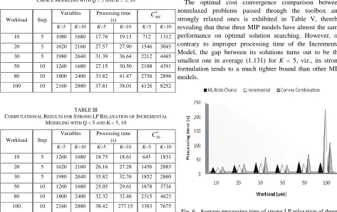
TABLEIII
COMPUTATIONAL RESULTS FOR STRONG LPRELAXATION OF INCREMENTAL
MODELING WITH Q=5 AND K=5,10
Workload Step
Variables Processing time
(s) CIN′
K=5 K=10 K=5 K=10 K=5 K=10
10 5 1260 1680 18.75 18.61 645 1831
20 5 1620 2160 26.16 27.28 1456 2883
30 5 1980 2640 35.82 32.76 1852 2860
50 10 1260 1680 25.05 29.61 1878 3734
80 10 1800 2400 32.32 32.46 2315 4623
100 10 2160 2880 38.42 277.15 3383 7675
TABLEIV
COMPUTATIONAL RESULTS FOR STRONG LPRELAXATION OF CONVEX
COMBINATION MODELING WITH Q=5 AND K=5,10
Workload Step
Variables Processing time
(s) CCC′
K=5 K=10 K=5 K=10 K=5 K=10
10 5 1260 1680 21.04 18.88 746 1799
20 5 1620 2160 30.36 39.45 1680 1968
30 5 1980 2640 55.42 35.45 2234 1685
50 10 1260 1680 27.77 30.34 2433 2042
80 10 1800 2400 66.13 83.16 3054 3601
100 10 2160 2880 109.12 133.23 4538 20330
The only significant variance between their solution approaches is their computational burden of performance. Fig. 6 represents the processing time of strong LP relaxations for three MIP models with K = 10 and Q = 5. These values are in the matter of seconds, whereas the optimal IP solution took about half an hour to get proved out in all likelihood. It is worth pointing out that the Incremental Model exhibits the worst solve time for the workload of 100, whereas the Multiple Choice Model [3] beats the Convex Combination Model, not touched on in there. We have conducted the experiments on a PC with i3 CPU of 2.13 GHz and 4 GB RAM running the Windows 7 64-bit operating system.
We employed the YALMIP as a complementary toolbox for MIP solving; getting integrated to the Matlab® built-in toolboxes. One of the basic ideas in YALMIP is to rely on external solvers for the low-level numerical solution of optimization problem. It concentrates on efficient modeling of high-level algorithms.
The optimal cost convergence comparison between nonrelaxed problems passed through the toolbox and strongly relaxed ones is exhibited in Table V, thereby revealing that these three MIP models have almost the same performance on optimal solution searching. However, on contrary to improper processing time of the Incremental Model, the gap between its solutions turns out to be the smallest one in average (1.131) for K = 5, viz., its strong formulation tends to a much tighter bound than other MIP models.
Fig. 6. Average processing time of strong LP relaxation of three MIP models with K = 10 and Q = 5.
Parameter k ij
w f1 H1 H2 H3
Range [1,10] [10,20] [5,10] (10,20] (20,40]
Parameter β1 β2 β3
Range [2,3] [1,
1
[image:5.612.64.537.428.725.2]TABLEV
OPTIMALITY TIGHTNESS FOR DIFFERENT STRONGLY RELAXED MIP MODELS WITH K=5 AND K=10
On the other hand, it is somehow remarkable that the Convex Combination Model is much likely the worst convergence case that is most important to bear in mind in view of its widespread applicability. These statements thus constitute worthy modeling inferences favoring one type of MIP models over the others.
VII. CONCLUDING REMARKS
In this paper, we considered a multistage PTP with piecewise linear transportation cost and nonlinear production cost. Three MIP models for solving PTP with strong relaxation adapting cutting-plane algorithm were sketched and run through. We distinguished that the disparity between the LP relaxation and the MIP is unlikely to be evident (less than 19%), and that the Multiple Choice Model outperforms other MIP models with respect to the computational complexity as the problem size and the number of commodities increase. We recommend constructing a globally dispersed multistage supply chain network with in-house production plants and outsourcing facilities that designates the PLCNF together with some extended forcing constraints through a so-called Lagrangean heuristic to bring out any improvement over the current work.
REFERENCES
[1] Guisewite, G. and P. M. Pardalos, “Global Search Algorithms for Minimum Concave Cost Network Flow Problems,” Journal of Global
Optimization, vol. 1, no. 4, pp. 309-330, 1991.
[2] Chu, L. Y., V. N. Hsu and Z. Shen, “An Economic Lot-Sizing Problem with Perishable Inventory and Economies of Scale Costs: Approximation Solutions and Worst Case Analysis,” Naval Research
Logistics, vol. 52, no. 6, pp. 536-548, 2005.
[3] J. Shu, Z. Li, and W. Zhong, “A production-transportation problem with piecewise linear cost structures”, IMA Journal of Management
Mathematics Advance Access, Jan. 2011.
[4] K. L. Croxton , B. Gendron and T.L. Magnanti , “A Comparison of Mixed-Integer Programming Models for Non-Convex Piecewise Linear Cost Minimization Problems”, Management Science, vol. 49, No. 9, pp. 1268-1273, 2003.
[5] Z. J. M. Shen, J. Shu, D. S. L., C. P. T. and J. Zhang, “Approximation Algorithms for General One-Warehouse Multi-Retailer Systems”,
Naval Research Logistics, vol. 56, no. 7, pp. 642-658, 2008.
[6] Vielma, J.P, S Ahmed and G Nemhauser, "Mixed-integer Models for Nonseparable Piecewise-Linear Optimization: Unifying Framework and Extensions," Operations Research, vol. 58, no.2, pp. 303-315, 2010.
[7] Croxton, K L, B Gendron, and T L. Magnanti, "Variable Disaggregation in Network Flow Problems with Piecewise Linear Costs," Operations Research Baltimore Then Linthicum, vol. 55, no. 1, pp. 146-157, 2007.
[8] Eksioglu, S. D., Eksioglu B. and Romeijn, H. E., “A Lagrangean Heuristic for Integrated Production and Transportation Planning Problems in a Dynamic, Multi-Item, Two-Layer Supply Chain,” IIE
Transactions, vol. 39, no. 2, pp. 191-201, 2007.
[9] Stecke, K. E. and Zhao, K., “Production and Transportation Integration for a Make-to-Order Manufacturing Company with a Commit-to-Delivery Business Mode,” Manufacturing and Service
Operations Management, vol. 9, no. 2, pp. 206-224, 2007.
[10] Bertsimas, Dimitris and J. N. Tsitsiklis. Introduction to Linear
Optimization. Belmont, Mass: Athena Scientific, 1997, ch. 3-7.
Workload
IN
C /CIN′ CMC/CMC′ CCC/CCC′ K=5 K=10 K=5 K=10 K=5 K=10
10 1.121 1.152 1.153 1.179 1.161 1.184
20 1.132 1.141 1.116 1.163 1.172 1.196