a b y z s0 c d w x s1 e f u v s2 g h s t s3 i j q r s4 k l o p s5 m n m n s6 o p k l s7 q r i j s8 s t g h s9 u v e f s10 w x c d s11 y z a b s12 a b y z s13 c d w x s14 e f u v s15 g h s t s16 i j q r s17 k l o p s18 m n m n s19 o p k l s20 q r i j s21 s t g h s22 u v e f s23 w x c d s24 y b
Representing pctl
Counterexamples
Master of ScienceThesis
Berteun Damman
Graduation Committee
Prof. Dr Ir Joost-Pieter Katoen
Tingting Han MEng (
韩婷婷
)
Dr Ir Arend Rensink
Abstract
Contents
Abstract v
Preface ix
0 Introduction 1
1 Preliminaries 5
1.1 Words and languages 5
1.2 Finite State Automata 8
1.2.1 History 8
1.2.2 An abstract automaton 8
1.2.3 The mathematical automaton 10
1.3 Regular expressions 12
1.4 Markov chains 13
1.4.1 Discrete Time Markov Chains 14
1.4.2 Paths in dtmcs 15
1.4.3 Probability of paths 16
1.4.4 Example dtmc 17
1.5 Computational Tree Logic 18
1.5.1 Syntax and semantics 19
1.5.1.1 Syntax 20
1.5.1.2 Semantics 21
1.6 Probabilistic ctl 22
1.6.1 Syntax and semantics 24
2 Counterexamples for pctl 25
2.1 Evidences and counterexamples 26
2.2 Conversion of the dtmc 30
2.2.1 Adaptation of the dtmc 30
2.2.2 Conversion to a weighted digraph 32
2.3 Finding the strongest evidence 34
2.3.1 Unbounded until 34
Contents
2.3.2.1 Reduction to an unconstrained problem 36
2.3.2.2 Hop constrained Bellman-Ford 39
2.3.2.3 Hop constrained Dijkstra 41
2.4 Finding the smallest counterexample 42
2.4.1 Unbounded until 43
2.4.1.1 Algorithmic description 44
2.4.2 Upper bounded until 46
2.4.2.1 Using dfs in the first phase 48
2.4.3 Double and lower bounded until 52
2.4.3.1 Algorithmic Description 55
2.4.4 Arbitrary bounded operators 56
2.4.5 Lazy algorithms 56
3 Implementation 59
3.1 Requirements and design goals 59
3.2 Program design 60
3.2.1 Language choice 61
3.2.2 dtmc and graph representation 61
3.2.3 Strongest Evidence algorithms 62
3.2.4 Smallest Counterexample algorithms 63
3.2.4.1 Alternative algorithms 65
3.2.5 Product graph construction 65
3.2.6 Regular expression 66
4 Experimental results 67
4.1 Synchronous leader election 68
4.1.1 The protocol 68
4.1.2 Mathematical analysis 69
4.1.2.1 The general case 70
4.1.3 More or less experimental results 71
4.1.4 Tables 72
4.2 Crowds protocol 72
4.3 Randomised mutual exclusion 78
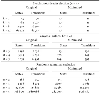
4.4 Bisimulation minimisation 79
5 Regular representations 85
5.1 From dtmcs to regular expressions. 86
5.1.1 Introduction 86
5.1.2 Formal definition 86
5.1.3 Evaluation of regular expressions 88
5.1.3.1 Interpretation of valuations 89
5.1.4 Regular expressions as counterexamples 90
5.1.5 Bounded expressions 93
Contents
5.2.1 Leader election example 94
5.2.2 Crowds protocol 95
5.2.3 Randomised mutual exclusion 97
5.3 Concluding remarks 97
6 Conclusion and future work 99
6.1 Conclusion 99
6.2 Future work 99
a ctl model checking 101
a.1 Outline 101
a.2 Time complexity102
b Counterexample explorer manual 103
b.1 Usage and requirements103
b.1.1 Example session104
b.2 Optional modules107
b.3 File formats108
b.3.1 Transition file108
b.3.1.1 Example file109
b.3.2 Labelling file 110
b.3.2.1 Example file 110
b.3.3 Formula file 112
c Acronyms 115
Index 117
Preface
The last miles takes the longest: this proverb summarises the whole process. It has been a long time since I have commenced my graduation. However, at last, the final product has been completed.
Because the subject is quite theoretical, and uses many mathematical ideas not familiar to most computer science students, and on the other hand uses quite some ideas from computer science not familiar to students of mathematics, this thesis contains a substantial introduction to the techniques used. I hope that this will make the ideas clear, since I do believe that the combination of mathematics and computer science in this area is very worthwhile, even tough during my study I have seen how many mathematical subjects have disappeared from the curriculum.
Finally I would like to thank my friends, parents and my graduation committee; and especially Joost-Pieter Katoen & Tingting Han, who gave me the opportunity to work on this subject in Aachen. Even though the ride was not very smooth at times, they were confident and willing to continue the supervision, even when I had my doubts.
As it turned out, they were right, and I am very grateful for this.
0
Introduction
The Dutch computer scientist Edsger Dijkstra, famous for his shortest path algorithm, once remarked in an interview with the Dutch news paperTrouw: ‘Software? By your leave, I think it’s rubbish.’1 He is clearly aggravated by the state of software and the number of times computers tends to crash.
And indeed, since the day the first computers have been built, and the first software was programmed, programmers and users alike have been plagued by bugs. Many strategies have surfaced to prevent, detect and repair these problems.
Some strategies rely on establishing ‘best practices’: rules of thumb which, if fol-lowed, avoid a number of common pitfalls; other strategies involve extensive testing of the written software against predetermined cases, in order to find the most common bugs. But as the same Dijkstra famously remarked: ‘Program testing can be used to show the presence of bugs, but never to show their absence!’
The field in which this thesis is written, is the field of formal methods. In this field the main strategy to prevent software bugs is called ‘model checking’. The model, a formal structure derived from an actual hardware or software design, is checked to see whether it obeys its formal specifications. This forms the core idea: verify aformal structure, againstformalspecifications. This verification is exhaustive. Every possible scenario should be verified. Verifying every possible scenario however, is very hard, and making it feasible to check ever larger and more complex systems is one of the challenges researchers in model checking face.
Because of the ability to mathematically verify software, and to guarantee the absence of errors, model checking is usually deployed in scenario’s in which correct behaviour of the software is of paramount importance, such as software for medical apparatus, space probes, flood barriers, and such. A notorious example of software errors leading to the death of three people is given by the Therac-25 radiation therapy machine, which would under certain conditions give massive overdoses of radiation. This underlines the danger of software errors in certain applications, and the important part model checking can play in preventing these mistakes.
The foundations of model checking were laid in 1981, by Edmund Clarke and E. Allen Emerson, initially developing model checking for hardware. As computers became more powerful, it became possible to also verify software models. In addition
1
0. Introduction
to the scenario described above, where faulty software can endanger lives, a new need for ensuring the correctness of software has emerged because of the proliferation of embedded software in all kinds of devices. Much software is located in places where patching is very expensive, such as in cars, and where a recall due to a software bug would be prohibitively costly for the manufacturer.
This has lead to the widespread adoption of model checking in both the hardware and software industries, and for this the Clarke and Emerson have been awarded the Turing Award2in 2007. Nevertheless, new techniques and refinements of existing techniques are constantly being discovered and developed, and this thesis tries to explore a small area of this large field even further.
Model checking thus aims to automate the process of finding bugs in software. Although knowing that software does not function according to the specification is useful, it is even more useful to be able to give a demonstration when it goes exactly awry. Only reporting ‘It doesn’t work’ will not aid the programmer much in ameliorating the problem. For this,counterexamplesare much more useful. These provide a sequence of steps after which the problem occurs. Such a sequence usually gives a clear indication where the software goes wrong, and which parts of the source code need to be patched.
Earlier theories of model checking allowed the specification and checking of prop-erties which stated that something bad would never happen, so calledsafety properties, or something good would always be the case, so calledliveness properties. For many practical applications such specifications are too rigid. Even if you backup your data every day to different computers in different countries, it could in theory still happen that in the same night each of these buildings burns down, and you lose your data. Since this is a very improbable scenario, most people are willing to take this risk.
Usually, we would like to know what risk we are taking exactly. A server equipped with multiple hard disks in a raid-configuration might fail irreparably if the rare situation occurs that after one disk fails a second one fails before the first one is replaced and rebuilt. Other questions could be that we want to guarantee a minimum level of service: if e-mail messages arrive randomly, but on average with a specific frequency, which might be higher during working hours, we would like to guarantee the mail server has enough capacity to always deliver nearly all messages within one minute, even if peak loads occur because by coincidence many messages are sent at the same time, in stead of evenly distributed. Finally, an example we shall see in this thesis too, in many distributed in which computers can join and leave a network, there has to be one computer that is designated the leader, electing such a leader occurs through some sort of voting process, but this can lead to a tie. If such a case, the computers have to vote again, by introducing a random factor in the vote, the election will be different next time, but we want to guarantee that ties do not occur too often, because as long as a leader has not been elected communication is usually suspended.
These are some very practical reasons why we are usually interested in questions such as ‘is the system able to respond within ten seconds 98% of the time?’ Or: ‘Will the availability be at least 99%?’ For this we need to be able to specify probabilities,
2
randomness and time-limits. A logic that allows us to specify this has been developed, and is calledpctl. Existing model checking algorithms forpctlare heavily based on the theory of Markov chains, which captures random and probabilistic behaviour and forms the underlying formal structure, and they are able to report whether a property is violated or satisfied by the model. In case it is violated however, these methods cannot provide the programmer with a counterexample. Algorithms that fill this gap have been designed recently.
The current algorithm works by finding a set of paths, which together form a counterexample. Roughly speaking, every path describes some scenario in which a problem occurs, and the probability of these scenario’s added together exceeds the specified limit.
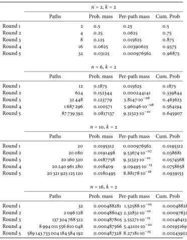
This thesis elaborates on the theory behind the algorithms, and describes a practical implementation of these algorithm which was made in order to get acquainted with the behaviour in practice. The obtained results show that in practice counterexamples will consist ofmanypaths. The number of paths will be so large that investigating them will be a daunting task.
The final chapters therefore will describe some preliminary ideas to reduce the size of these counterexamples, using regular expressions, or to present them in a form which can be more easily digested by the programmer.
Furthermore some remarks are made with respect to the algorithms used, and the possibility to achieve the same results by transforming the underlying transition structure instead of adapting the algorithms for certain verification problems involving bounded temporary operators.
1
Preliminaries
This chapter intends to serve as a reminder for those already familiar with the concepts used in this thesis, or as a primer for those unfamiliar with these concepts; the latter might want to refer to some of the textbooks mentioned, if they wish to acquire a more intimate knowledge of these subjects.
Those already knowledgeable of finite state automata, Markov chains or any of the other subjects introduced in this chapter might still want to glance over the material in order to get acquainted with the syntax used.
Although the reader can choose to only read those section wherewith he is not familiar, he or she should note that they were written to be read in sequential order, and will assume knowledge of the material in the previous sections.
A basic mathematical understanding, especially with respects to sets, is expected. Those unfamiliar with this should turn to a text book such as (Sudkamp, 1998) (especially the first chapter) or Wikipedia for an explanation of the concepts involved.
1.1 Words and languages
The termlanguagedescribes several distinct, yet related concepts. First of all there are languages such as English, German or Dutch, so callednatural languages. Furthermore there arecomputer languages, a rather specific set of symbols which can be used to write computer programs. Then there are alsosign languagesfor the deaf in which words are represented by gestures.
Speaking in an abstract manner, these languages share a common concept of symbols which can be combined to form words. In the case of English or Latin these are simply the twenty-six letters of the Latin Alphabet:a,b, et cetera. German adds some other symbols such asäandß. Greek and Russian even use a completely different set of symbols, whereas sign language uses gestures. Chinese has an enormous collection of basic symbols.
1. Preliminaries
This general idea that an utterance in a language consists of words which are in turn formed by symbols is the way language is defined in a theoretic way.
Definition 1.1.1. Analphabetconsists of a finite set of symbols, also called letters. We usually use Σ to denote the alphabet of a language.
Definition 1.1.2. Aword(also calledstring) is formed by juxtaposing a finite sequence of letters from an alphabet Σ. That is: w = a1a2⋯anwithai ∈ Σ. Its length is the
number of symbols, usually denoted as∣w∣.
Example 1.1.3. For example, consider the alphabetB= {0, 1}. Examples of words over
this alphabet are 001, 10001, 0, with respective lengths of three, five and one.
There also is anempty wordwhich has a length of zero, and this is denoted byε. Although words are considered to be indivisible units in a language, just as the word ‘symbol’ cannot be split in ‘sym’ and ‘bol’, we will allow definitions such asv =wa1
wherew is a word, anda1is a letter from Σ. We also allow ‘glueing’ of two words together, which is more precisely defined in the following definition:
Definition 1.1.4. Ifvandware words over an alphabet Σ, with:
v=a1a2⋯an w=b1b2⋯bn
The notationvwis used as a shorthand for:
vw=a1a2⋯anb1b2⋯bn
This is called theconcatenationofvandw. Ifwis the empty wordε, thenvw=vε=v,
and also ifvis the empty wordvw=εw=w.
Definition 1.1.5. If a wordwcan be written as the concatenation of two wordsuandv, i.e.w=uv, (with possiblyu=εorv=ε), we say thatuis aprefixofw, andvis a suffix
ofw. If there exists someuandvsuch thatw=uxv, we say thatxis asub-wordofw. Note thatεandwitself are always a prefix, suffix and sub-word ofw. Aproper prefix u ofwis a prefix ofw, whereu≠εandu≠w. Proper suffixes and proper sub-words are
defined analogously.
Using the empty word and this notation of concatenation we can give a definition of the set of words over Σ, which henceforth will be denoted as Σ∗.
Definition 1.1.6. The set of words over Σ is recursively defined as follows:
1. ε∈Σ∗, this is the basis.
2. Ifw∈Σ∗anda∈Σ, then alsowa∈Σ∗; this forms the recursive step.
3. Only those words formed by a finite number of applications of the previous two steps are in Σ∗
Example 1.1.7. Let Σ= {a,b}. Using the previous definition we can list the elements
1.1. Words and languages
Length 0 ε;
Length 1 a,b;
Length 2 aa,ab,baandbb;
Length 3 aaa,aab,aba,abb,baa,bab,bba,bbb.
We see that there will be 2kwords of lengthkfor this alphabet. In general we see that for an alphabet consisting ofnsymbols there will benkwords of lengthk.
Similar to the English language, not every possible word that can be formed is considered a valid English words (such asxuqa). A language will normally have some restrictions on the set of all possible words, thus restricting the language to a subset of all possible words. This is expressed in the following definition.
Definition 1.1.8. Alanguageover an alphabet Σ is a subset of Σ∗.
This need not be a proper subset, for the language of non-negative numbers is formed by all words over the alphabet{0, 1, 2, . . . , 9}. The language consisting of all prime
numbers however, is a subset of the words over the alphabet{0, 1, 2, . . . , 9}. The word
32 is not part of this language, but 13 and 71317 are. The latter would even be part of the more restricted language of palindromic primes.
One can also have more than one language over the same alphabet of course. One could for example define the language ‘even numbers’, and the language ‘multiples of three’ over the alphabet{0, 1, 2, . . . , 9}.
Languages themselves, similar to words, can also be combined in different ways to create new languages. Two languagesL1andL2can be merged into a new languageL:
L = L1∪ L2, which defines the language of all words either inL1or inL2or both.
Two languages can also beconcatenated, this is written as
L1L2= {w1w2∣w1∈ L1andw2∈ L2}
Example 1.1.9. Suppose we would have a languageL1 = {over,under}and another
language with the wordsL2 = {achieve,coat,sea}, then the concatenation of these
languagesL1L2would consist of the six (British) English words{overachieve,overcoat,
oversea,underachieve,undercoat,undersea}.
Commonly though, this construct is used to expand a set of letters to a language consisting of all words that can be formed by these letters; by repeatedly concatenating the language to itself, which we shall see below.
This way, also thepowerof a language can be defined. Then-th power of a language
Lis written asLn, wherenis a non-negative integer, and is defined as follows:
1. L0= {ε}
2. Ln=Ln−1L, forn>0.
A final, important, operation, is the (Kleene)starorKleene closureof a language, which is written asL∗and defined as:
∞
⋃
i=0
1. Preliminaries
Note that the notation Σ∗is consistent with this.
Now that we have stipulated what is meant by words and languages we can advance to the concept of a Finite State Automaton (fsa).
1.2 Finite State Automata
1.2.1 History
Finite state automata can be found at the heart of theoretical computer science. Despite this theoretical character, their practical applications are surprisingly wide ranging and manifold.
The roots offsas can be traced back to the work of Warren McCulloch and Walter Pitts, whose article, (McCullo ch & P it ts,1943), described a mathematical model of neurons, i.e. nerve cells in the brain. Even though Alan Turing had presented his Turing machine seven years before, and as such had introduced the idea of an abstract machine performing in a deterministic manner, his machine is way more powerful than a finite state automaton.
The work of McCulloch an Pitts was subsequently presented to Stephen Kleene for investigation by the rand corporation. This research, although completed in 1951, was not published until 1956. His seminal work (Kleene,1956) also provides a proof of what is now known as ‘Kleene’s theorem’, a result linking regular sets and finite state automata intimately.
During the following years the theory behindfsas has been greatly expanded andfsas have been applied in many fields, partly because of their simplicity which gives them a large practical advantage over Turing-machines, whose properties are mostly studied in an abstract context.fsas however are very useful in solving problems involving circuit design, lexical analysis and text processing and in recognising certain numbers or even biological sequences.
The interested reader, with a command of the French language is referred toP er-rin(1995) for a more detailed exposition of the history offsas.
1.2.2 An abstract automaton
fsas are usually used to determine whether a word belongs to a language, i.e. a subset of all possible words (or strings) over a given alphabet. The language of even numbers over the alphabet of digits will only consists of digits ending in 0, 2, 4, 6 or 8. Something like 13 is a valid word, but it is not part of the language of even numbers. It turns out that for certain languages one can construct anfsa, whereas one cannot for other. The languages for which one can construct anfsaare calledregular languages.
There are several ways to depict automata, as a picture with circles and arrows or in a more mathematical way. We shall start out with the pictures, which give a more intuitive idea, and will then provide the mathematical definition.
1.2. Finite State Automata
s t
1
0 0
1
Figure 1.1 An automaton accepting words over{0,1}, ending with 0.
of the states of the automaton. When the automaton ‘runs’ it will move from state to state, obeying the arrows in the figure. If there is an arrow from one state to another, that means the automaton can make atransitionfrom the first state to the next one, provided the input matches the symbol near the arrow. For example, the automaton in
figure 1.1can make a transition fromstotprovided the input is 0. It can return tos fromtin case of a 1 in the input. Also, it can stay int, if another 0 is input.
The input is usually a word, in the sense defined indefinition 1.1.2. The automaton will consume this word symbol by symbol, and take the appropriate transition. It will start reading from the left, so if the word 001 was provided to our sample automaton at the moment it was ins, it would move tot, consuming the first 0, and leaving 01 to be processed. After that it would consume another 0, which means it will stay intand finally it would see a 1, so it would return tos. If the automaton would reside intat the moment it was given 001 it would also end up ins.
To make clear where an automaton starts, a special state, called aninitial state exists, which is designated as . Infigure 1.1this is states. Also, there is at least one
final statein the automaton, which is indicated by a circle with a double border: , which is statetin the example.
If the automaton ends in a final state after having consumed the final symbol of the input word, it is said toacceptthis word. Our example automaton will thus accept any word consisting of zeros and ones, ending with a zero. One could interpret these words as binary numbers and say that it will only accept those numbers ending with 0, or indeed the even numbers.1
In the real world, many automata also take some form of input. In the case of vending machines, this will consist of some coins, which need to add up to the required amount; or in case of a combination lock it should be a series of digits that have to be input in the right order. One can also model these automata as anfsa. In the first case the alphabet will for example consist of the symbols €0.10, €0.20 and €0.50, if the automaton only accepts ten, twenty and fifty cent coins. A ‘word’ is a sequence of these symbols. One can see infigure 1.2athat the words that are accepted are those that have a monetary value of €0.50. In case of the combination lock, shown infigure 1.2bthe winning combination is 642, which has to be input in the right order.
1
1. Preliminaries
€0.50 €0.40 €0.30 €0.20 €0.10 paid
€0.50
€0.10
€0.20 €0.10
€0.20 €0.10
€0.20 €0.10
€0.20 €0.10
aA model of a vending automaton, which accepts exactly €0.50 in coins of €0.10, €0.20 or €0.50.
s 6 s1 4 s2 2 open
b A model of a combination lock. This is like peering inside the lock – in reality one would only be able to try to input something and see whether the automaton accepts it.
Figure 1.2 Two examples of finite state automata, based on ‘real world’ automata.
One could wonder, what if someone inputs a symbol which is not defined for that state? For example, someone inputs a 3 in the combination lock. In fact this is negligence on our part, a truly deterministicfsashould have exactly one transition at every state for every possible input symbol. Usually it is made implicitly clear what to do if a symbol is not defined, in the case of the combination lock it should start over, in other cases the automaton might be amended to include one extra state, to which every ‘undefined’ transition will go. Once having entered this state, the automaton will stay there and make a transition to itself for every possible input symbol.
One can see how an automaton accepts a word, and we know that a language consists of words. Noting this, we can see how an automaton also describes a language, viz. the language of those words accepted by the automaton, which is usually a subset of all words over the (input) alphabet of the automaton. The ‘language’ of the vending machine consists of input sequences that added up are worth €0.50. The language of the combination lock are only those sequences that end in 642, out of all possible sequences of integers.
We will make this connection more precise and formal in the next section.
1.2.3 The mathematical automaton
The previous section presented a rather intuitive model of the automaton, and a way to visualise it, using circles and arrows. Now we shall provide a mathematical definition. This mathematical definition formalises and specifies what is meant exactly when we mean by accepting a word.
The previous section however, can always be used as an intuitive guidepost.
Definition 1.2.1. AFinite State Automatonis defined as a quintuple(Σ,Q,I,F,E),
1.2. Finite State Automata
finally the edges are given byEsuch thatE⊂Q×Σ×Q.
Definition 1.2.2. A deterministicfsais anfsawith the following constraints:
◆ ∣I∣ =1, i.e. there is a unique initial state.
◆ For each pair(s,a) ∈Q×A, there is at most one statet∈Qsuch that(s,a,t) ∈E,
i.e. in every state there is at most one choice for a given input symbol.
The automata in thefigure 1.1and figures1.2aand1.2bare all deterministic. In the combination lock example however, we did not specify what should happen if the user tries to input 4 in states. Automata like this one, which do not specify an action for every input symbol in every input state are called incomplete, a notion specified in the next definition.
Definition 1.2.3. Anfsais calledcompleteif for each pair(s,a) ∈Q×A, there is at
least one statet∈Q, such that(s,a,t) ∈E. i.e. in every state there is at least one choice
for a every given input symbol. If there is no option for some input symbol from the symbol, the automaton is calledincomplete.
Now that we know what an automaton looks like mathematically speaking, we can make the concept ofaccepting a wordmore precise. But first we need to define how we associate words with automata.
Definition 1.2.4. Apathin an automatonA = (Σ,Q,I,F,E)is a sequence of connected
edgesp=e1⋯en, whereei = (si,ai,ti) ∈E, such thatti =si+1, fori<n. The statesi will be called thesourceof the path and the statetnwill be called theendof the path.
The ordered concatenation of the symbolsai, i.e. a1⋯angives thelabelof the path.
This label is also a word, compare withdefinition 1.1.2.
Having established how we associate a word with a path in a automaton the time is ripe to give a definition of accepting a word.
Definition 1.2.5. An automatonA = (Σ,Q,I,F,E)is said toaccepta wordwif there
is a path inAwith labelwsuch that its source is an element ofIand its target is an element ofF. Such a path is calledsuccessful.
The previous definitions enable us to straightforwardly give a definition of the language of an automaton:
Definition 1.2.6. Thelanguageof an automatonA, written asL(A)is defined as the
set of all words accepted byA.
1. Preliminaries
s t
0, 1
0
Figure 1.3 A non-deterministic automaton accepting words over{0,1}, ending with 0.
The following theorem, which is given without its (short) proof states this is not the case – the interested reader is referred to (Sudkamp,1998) or (P errin,1990) for details.
Theorem 1.2.7. For each finite automaton, there exists a deterministic and complete finite automaton which accepts exactly the same language.
In practice however, it is often much easier to specify an incomplete automaton (as we have done in the examples in figure1.1,1.2aand1.2b), and at times a lot more concise to specify a Non-Deterministic Finite State Automaton (nfa). Although we have not paid much attention tonfas, the main difference with a Deterministic Finite State Automaton (dfa) is that for annfawhich accepts a wordwthere might be other paths with the same label that are not successful. This does not matter as long as there is at least one path that is successful. An example of a slightly more compact specification of the automaton infigure 1.1is given infigure 1.3. For the input symbol 0 there are two choices in states. Either stay ins, or go tot. The ‘right thing’ to do is to only choose the transition totif the 0 is the last symbol of the input. The automaton of course does not know this, it is not supposed to be clairvoyant. It has to decide in an ad-hoc manner what to do with the current input symbol. If one wishes, one could interpret it as always choosing the correct option, or as exploring every option in parallel. Our definition however, only states that there should exist some successful path for this word; how this path is to be found in practice is immaterial.
1.3 Regular expressions
The previous section described the wayfsas relate to languages and words in the sense we have defined them. As implied therein, there are many different ways to define which words can be part of a language, but one of the simplest ways, known to linguists as a ‘Type 3 grammar’ is given by regular expressions.2
It turns out that these regular expressions give another method to define regular languages. Becausefsas can also be used to define regular languages, these two formalisms are equivalent. Every language for which one can construct an automaton, one can also define by a regular expression.
2
Some authors, especially from the Francophone parts of the world, prefer the termrational expres-sion, because of the close analogy between these expressions and the rational power series (or fractions)
1.4. Markov chains
Definition 1.3.1. Let Σ be an alphabet. The set of regular expressions over Σ is recurs-ively defined as follows:
1. εand∅are regular expressions.
2. For every symbola∈Σ,ais a regular expression.
3. Ife1ande2are regular expression, then so aree1e2,(e1+e2)and(e1∗).
4. Nothing else is a regular expression.
Normally, the parentheses are not always written down. For example, an expression like
aε+bc∗should be read like((aε) + (b(c∗))). From this we can see concatenation has
precedence over+, but∗has precedence over concatenation. A frequently encountered
variant notation fora+bisa∣b.
The regular expressionsaandεrepresent the languages which just consist of that single symbol. An expression likee1+e2represents a choice, it represents the union of
the languages defined bye1ande2. The∗represents repetition, and is a shorthand for all strings in which the previous symbol is repeated zero or more times.
Definition 1.3.2. The languageL(e)defined by a regular expressioneis as follows
L(∅) = ∅ L(ε) =ε
L(a) = {a} L(e1e2) = L(e1)L(e2)
L(e1+e2) = L(e1) ∪ L(e2) L(e∗) = L(e)∗
Kleene(1956) first proved the equivalence of regular expressions andfsas. There furthermore exist different methods to convert a regular expression to anfsawhich accepts the same language as the regular expression defines, and vice versa. An overview of the different approaches can be found in the article byYu(1997).
1.4 Markov chains
The field of Markov chains is mathematically very well developed, and knows many applications in the fields of biology, physics and also computer science. They are named after the Russian mathematician Andrei Markov (Андрей Марков).
A Markov chain, in a way, can be viewed as some sort of autonomous automaton, which starts in a certain state, and then moves with some probability to another state by itself. It hence differs from a normal automaton by not requiring input, like the vending machine example offigure 1.2a. Instead, it makes the transitions according to a certain probability. The defining property of the Markov chain is that this probability of going from a certain states1to a states2, only depends on the current state the automaton is in, and not on any previous state it might have visited, this is known as theMarkov
property. Finally, the Markov chain does not have an accepting state.
1. Preliminaries
start→headsshould have a probability of 1⁄2 , and hence the transition totailsshould
also have probability 1⁄2 . Indeed, every transition should have probability 1⁄2 in this automaton.
This expresses, that even though one might have flipped heads already ten times, the probability that heads will come up after the next flip does not change, as we expect, because the coin does not have any memory.
For example, many games, such as Monopoly, can be viewed as Markov chains. The square a player will land on will solely depend on the square its currently on and the outcome of the next throw.3Other games, such as Blackjack, cannot be modelled as a Markov chain, since the probability that you won’t exceed 21 if you already have 17 depends on the cards already drawn during previous turns.
Mathematically, a Markov chain is usually represented as a transition matrix. That is, an entrypi jin the matrix represents the probability of going from stateito state j. Furthermore, the probabilities in every row should add up to one, i.e.∑jpi j =1,
because you always have to go to some other state (or stay where you are). A matrix in which every row adds up to 1 is calledstochastic.
The namechainmeans the state space of the Markov process is finite. The process is defined as a sequence of random variablesX1,X2, . . . which indicate the state for each moment in time, with the Markov property which states that the next state solely depends on the present state and not on the previous state, or formally:
Pr(Xn+1=x∣Xn=xn, . . . ,X1=x1) =Pr(Xn+1=x∣Xn=xn).
Note that we have also tacitly assumed that Pr(Xn+1=x∣Xn=xn) (the one step
probabilities) are independent ofn, which means the transitions probabilities are
stationary. This assumption allows us to arrange the transition probabilities as a matrix.
1.4.1 Discrete Time Markov Chains
To be precise, the Markov chains we use are Discrete Time Markov Chains (dtmcs)4. In the following definition, letAPdenote a fixed, finite set of atomic propositions. We usually usea,b,c, . . . orai to denote these propositions. Their rôle is semantic.
For example, the atomic propositionhmight indicate an outcome ‘heads’ for the coin toss example. Orsuccessmight indicate some operation has succeeded. We use these propositions to annotate states; the next section will make use of these propositions.
Definition 1.4.1. A (labelled) Discrete Time Markov Chain (dtmc) is a tripleD = (S,P,L), where:
3
After the throw, one might land on Community Chest, or Chance, thus moving again, but assuming you pick a random card from the pile in each case, this can be modelled very simply. Suppose you have to throw 5 to arrive at Chance. This has a probability of 1⁄9 . Then, there is probability of 1⁄16 you pick the ‘Advance to Go’ card, and hence for that turn there is a probability of 1⁄144 of ending at Go, assuming you couldn’t arrive at it directly.
4
1.4. Markov chains
◆ Sis a finite set of states;
◆ P∶S×S→ [0, 1]is a stochastic matrix;
◆ L∶S→2APis a labelling function which assigns to each states∈Sthe setL(s)
of atomic propositions that are valid ins.
Note that, from a computer scientist’s point of view, adtmcis a Kripke structure in which all transitions are equipped with discrete probabilities such that the sum of the outgoing transition probabilities of each state is equal to 1.
Note also, that we do not equip thedtmcwith a starting distribution, in this thesis we always assume thedtmchas a unique initial state.
IfP(s,s) =1 fors∈S, then we call that stateabsorbing. If we draw thedtmcas a
picture, we do not draw the transitions between statess1ands2for whichP(s1,s2) =0.
Thesizeof adtmcDis denoted by∣D∣, and is the number of non-zero entries inP.
1.4.2 Paths inDTMCs
Having established what adtmcis, and how to give certain properties to states using atomic propositions and a labelling function, we shall now make clear how to specify a sequence of movements ‘through’ adtmc.
Definition 1.4.2. LetD = (S,P,L)be adtmc.
◆ An infinitepath σ inD is an infinite sequence s0s1s2⋯ of states, such that ∀i ≥ 0∶ P(si,si+1) >0.
◆ Afinitepath is a finite prefix of an infinite path.
Note that, becausePis stochastic we can never get stuck in a state, every state has a successor. An infinite path is thus always possible. Because there is only a finite number of states in the structure, an infinite path needs to have some parts that are repeated infinitely often, we use theωsubscript for this, e.g.s1s2(s3s4)ωindicates a path where
the suffixs3s4is repeated infinitely often at the end of the path.
We usePathsD(s)to denote the set of all infinite paths inDthat start in statesand
we usePathsDfin(s)to denote the set of finite paths starting ins. If it is clear from the
context whichDis meant, we omit the superscript.
Let ˆσ=s0⋅s1⋯sn∈PathsDfin(s0). That is, ˆσis a finite path starting ins0. IfP(sn,s) >
0, then we can extend a pathσ bys, which we denote asσ⋅s. The length of a path
σ is denoted as∣σ∣and is measured by the number oftransitionsof a path. Hence,
∣σˆ∣ = ∣s0s1⋯sn∣ =n, and∣s∣ =0. For an infinite pathσwe have∣σ∣ = ∞.
There are also some operators for obtaining a specific state in a path, and for obtaining the prefix or suffix of a path. Indexing starts at 0, so we writeσ[i]to obtain
the(i+1)-th state in the path, with 0≤i ≤ ∣σ∣. So, for example, ˆσ[i] =si. Letσ[≤i]
denote the prefix of pathσtruncated at lengthi, thus ending at the(i+1)-th state. That
isσ[≤i] =σ[0]σ[1]⋯σ[i]. Dually, the suffix of a path, written asσ[≥i]is defined as
1. Preliminaries
The set of all prefixes of a pathσis denoted asPref(σ)with:
Pref(σ) =
∣σ∣
⋃
i=0
{σ[≤i]}
1.4.3 Probability of paths
Now that we have a way of specifying paths in adtmc, where every transition has a certain probability associated with it, we would like to assign a probability to the whole path. That is, the probability that these transitions actually occur.
For this we make a small sidestep into measure theory, but this is only for the theoretical foundations, since the measure itself is as we would intuitively expect.
When looking from a probabilistic point of view, terms likeexperiment,outcome andevent are used. For example, the experiment might be a throw of a dice, the outcomes would be 1 to 6, and an event could be throwing an odd number, which would be an outcome of 1, 3 or 5. So basically events consist of a set of outcomes.
Withdtmc, the experiment is arunthrough thedtmc; that is to say: we start in our initial state, then go to a successor state, again, and again. The outcome of such a run will be a path, in the sense ofdefinition 1.4.2. Because paths are infinite, the probably that a specific single path will occur can be zero, for example the probability of infinitely often throwing heads is zero.5 This is why we are usually interested in events that consist of an (infinite) set of paths. We use the set of finite paths as as basis. The reason for this is that generally we are in something happening within a finite amount of time, and after that the course of the path is irrelevant for us.
This leads us to the idea of a (basic) cylinder: namely the set of all paths that start with a specified prefix.
Definition 1.4.3. Thecylinder setof a finite path ˆσ=s0⋅s1⋯sn∈PathsDfin(s0)is defined
as:
Cyl(σˆ) = {σ∈PathsD(s0) ∣σˆ∈Pref(σ)}
These cylinder sets play an important part in what we consider an event in the context ofdtmc. The probability of an event comprising of a single cylinder set can now simply be found by multiplying the probabilities of the transactions in the prefix that generated the cylinder set. That this should indeed be a valid probability, can intuitively be seen by considering that the only thing that matters is that the prefix occurs, after that any continuation is good. The probability that something happens is 1. Hence, the probability for the whole set is given by the prefix.
We complete this interlude with a formal definition of the informal exposition above. The reader who is interested in a more thorough discussion of the ideas presented
5
1.4. Markov chains
a A mouse in a maze with cheese and an exit.
start
{s}
c1
∅
free
{f}
cheese
{c}
exit ∅ c2 ∅ c3 ∅ 12 14 14 14 14 13 13 25 25 14 12 12 1 13 15 14 14 34
b The corresponding transition sytem.
Figure 1.4 An example of a maze and theDTMCmodelled after it.
here is referred to the article by Panangaden (2001) or the book ofBaier & K atoen(2008, chapter 10). In addition,Capinski & Kopp(2004) provides a basic introduction into probability and measure theory, and explains for example what a
σ-algebra is, which we use without further explanation in the following definition.
Definition 1.4.4. The probability measure PrD
s0(briefly Pr) induced by adtmcDwith
initial states0is the unique measure on itsσ-algebra:
Pr{σ ∈Paths(s0) ∣s0⋅s1⋯sn∈Pref(σ) ´¹¹¹¹¹¹¹¹¹¹¹¹¹¹¹¹¹¹¹¹¹¹¹¹¹¹¹¹¹¹¹¹¹¹¹¹¹¹¹¹¹¹¹¹¹¹¹¹¹¹¹¹¹¹¹¹¹¹¹¹¹¹¹¹¹¹¹¹¹¹¹¹¹¹¹¹¹¹¹¹¹¹¹¹¹¹¹¹¹¹¹¹¹¹¹¹¹¹¹¹¹¹¸¹¹¹¹¹¹¹¹¹¹¹¹¹¹¹¹¹¹¹¹¹¹¹¹¹¹¹¹¹¹¹¹¹¹¹¹¹¹¹¹¹¹¹¹¹¹¹¹¹¹¹¹¹¹¹¹¹¹¹¹¹¹¹¹¹¹¹¹¹¹¹¹¹¹¹¹¹¹¹¹¹¹¹¹¹¹¹¹¹¹¹¹¹¹¹¹¹¹¹¹¹¹¹
Cyl(s0⋯sn)
} =
n
∏
i=1
P(si−1,si). (1.1)
Theσ-algebra should be the smallestσ-algebra containing all cylinder sets induced by the finite paths starting ins0.
By slight abuse of notation we also write Pr{σ}as a shorthand for Pr{Cyl(σ)}, where
σis a finite path.
1.4.4 ExampleDTMC
We shall now present an example of a situation which can be modelled by adtmcto elucidate the terminology introduced in the previous sections.
1. Preliminaries
there is a piece of cheese6. If the mouse discovers this, it will be less inclined to go to another room. If the mouse escapes, it will never come back in the maze.
Infigure 1.4b, the corresponding transition system is shown. If a cell has two exits to another cell, the mouse is more likely to end up in this cell. We can see that ‘free’ is an absorbing state. This means that eventually, the mouse will always find the exit. Although, of course, in theory the mouse could decide to always stay in the first room, the probability of this is negligible.
A finite path in this maze could beσ1 = start⋅c1⋅cheese⋅cheese. An infinite path
might beσ2=start⋅c1⋅c3⋅c2⋅exit⋅(free)ω
The probability of the first path, Pr{σ1}, can be found by multiplying the
probabil-ities on the transitions: Pr{σ1} =12⋅14⋅34=32 . If we would formally define a3 dtmcfor
this transition system, sayD = (S,P,L), we would have:
◆ S= {start,cheese,exit,free,c1,c2,c3}
◆ For the transition matrix (which uses the same order for the states as the previous item) we have:
P= ⎡ ⎢ ⎢ ⎢ ⎢ ⎢ ⎢ ⎢ ⎢ ⎢ ⎢ ⎢ ⎢ ⎢ ⎢ ⎣
12 0 0 0 12 0 0
0 34 0 0 14 0 0
0 0 13 13 0 13 0
0 0 0 1 0 0 0
14 14 0 0 14 0 14
0 0 25 0 0 15 25
0 0 0 0 14 12 14
⎤ ⎥ ⎥ ⎥ ⎥ ⎥ ⎥ ⎥ ⎥ ⎥ ⎥ ⎥ ⎥ ⎥ ⎥ ⎦
◆ And the labelling function is defined as: L(start) = {s}, L(cheese) = {c},
L(free) = {f}. For the other nodes we haveL(⋅) = ∅.
1.5 Computational Tree Logic
Computational Tree Logic (ctl) (Cl arke & Emerson,1981) is defined as a propos-itional branching-time temporal logic. As it is one form of temporal logic, it fits in the larger framework of modal logic; in this thesis however, we only concern ourselves with
ctlas far as necessary for an understanding of the material involved here.Emerson (1990) provides a more detailed account on various temporal and modal logics.
Being atemporallogic,ctlallows us to propose things that will happen as time passes. For example, if someone is flipping a fair coin, one can state: until you flip heads, you flip tails. The previous will of course happenalways, but you could also propose that ‘you will eventually flip two heads and two tails’ in a row. This need not happen, for one could, in theory, flip only heads, or flip heads and tails alternately.
Being abranchingtemporal logic,ctlallows us to view time, and in particular the future, as a tree of possible scenario’s. That is, to continue the coin flipping example, first one might flip heads, and then one might flip heads again, and then tails. Or perhaps
6
1.5. Computational Tree Logic
start
heads
tails heads
tails
tails heads
tails heads
aAn automaton representing an infinite sequence of coin flips.
(start, 0)
(heads, 1)
(heads, 2)
(h, 3)(t, 3)
(tails, 2)
(h, 3)(t, 3)
(tails, 1)
(heads, 2)
(h, 3)(t, 3)
(tails, 2)
(h, 3)(t, 3)
b An infinite sequence of coin flips as an infinite tree (h = heads, t = tails)
Figure 1.5 A finite structure and the corresponding unwound infinite tree.
one would start with tails, et cetera. Viewed thusly, one could draw an infinite tree of scenario’s. Such a tree can be derived by unwinding a finite structure, for example an automaton. An example of this idea is given infigure 1.5, where one sees an automaton and its corresponding tree.
Also, one can see in thefigure 1.5bthat time is represented as a discrete sequence of events. This allows us to speak about ‘the next moment in time’, or ‘within five moments’; meaning we speak about the next level or the next five levels in the tree. Furthermore, we can clearly see how many scenario’s there are. There are, for example four different ways to arrive at the second level in the tree, where each node represents a different sequence of coin flips.
The important aspect when employing temporal logic, is that one tries to reason about the behaviour of an underlying system which possibly never ceases running. These systems are typicallyreactive. They wait for some input, move to another state, and wait for input again. Other methods for program verification are often based on thetransformationfrom one state to another, and one proves that this transformation is executed correctly, and after the computation the program is done. An example of this is a compiler which takes an input file and outputs an executable or a formatted document. An operating system however can keep on running and reacting to messages from the keyboard and the network.
The next section will define the syntax and semantics in a more thorough and mathematical way. Note that, although the semanticsctlcan be defined more generally for any transition system (or semi-automaton), we use thedtmcs described in the previous section as the underlying structure.
1.5.1 Syntax and semantics
Sincectlis a branching logic, there is more than one scenario for the future. Its operators reflect this fact. One can quantify over these different scenario’s – or paths. There are the basic temporal operatorA(for all futures) andE(for some future); these
1. Preliminaries
(next moment),U(until) andW(unless). These linear time operators do not view time as branching, these are applied to one specific future scenario or path; the branching aspect ofctlis provided by theAandEoperators. A combination likeEFwin lottery
intuitively might have the meaning ‘I might potentially win the lottery.’ Sadly enough, this is not the guaranteed possible future, and it is not very probable it will be ours. The morbidAFdieexpresses that whatever the future will be, it is inevitable that we die
some time. We furthermore allow for a bound on the maximum number of moments that can pass before something should hold, for exampleAG≤3rainmight be interpreted
as a bad weather forecast which states that ‘for the next three days it will invariantly rain’. If the bound is not mentioned, it is taken as being infinite and calledunbound.
The inclusion of a time-limit on the operators was independently proposed by (Emersonet al.,1991) and (Hansson & Jonsson,1994). The latter also introduced a probabilistic operator, thus describing what is known as Probabilistic Computational Tree Logic (pctl), which will be described in the next section.
1.5.1.1 Syntax
Definition 1.5.1. We again use an inductive definition. LetAPthe set of propositions. First we give the state-formulae:
1. For everya∈APwe have:ais a state-formula.
2. If Φ is state-formula, then¬Φ is a state formula.
3. If Φ and Ψ are state-formulae, then Φ∨Ψ is a state-formula.
4. Ifφis a path-formula, thenEφandAφare state-formulae.
5. Only those formulae formed by a finite number of applications of the previous four steps are state-formulae.
Path formulae are formed by the following rules:
1. If Φ is a state-formula, thenXΦ is a path formula.
2. If Φ and Ψ are state-formulae, then ΦU≤hΨ, withh∈N∪ {∞}is a path-formula.
3. If Φ and Ψ are state-formulae, then ΦW≤hΨ, withh∈N∪ {∞}is a path-formula.
4. Only those formulae formed by a finite number of applications of the previous three steps are path-formulae.
Remark1.5.2. In stead ofU≤∞andW≤∞we simply writeUandW. These operators are
also calledunbounded, whereasU≤handW≤hwith 0≤h≤ ∞are calledbounded.
Other logical connectives, such as Φ∧Ψ or other temporal operators, such asFΦ can
1.5. Computational Tree Logic
equivalences hold
tt≡Φ∨ ¬Φ EF≤hΦ≡E(ttU≤hΦ)
ff≡ ¬tt AF≤hΦ≡A(ttU≤hΦ)
Φ∧Ψ≡ ¬(¬Φ∨ ¬Ψ) EG≤hΦ≡E(ΦW≤hff)
Φ⇒Ψ≡ ¬Φ∨Ψ AG≤hΦ≡A(ΦW≤hff)
Φ⇔Ψ≡Φ⇒Ψ∧Ψ⇒Φ AXΦ≡ ¬EX¬Φ
1.5.1.2 Semantics
In order to give the formulae some meaning, apart from the intuitive idea, we define two satisfaction relations (both denoted by⊧). The first is for the path-formulae, and
the second one for the state-formulae. Remember, we use thedtmcs described in the previous section as our underlying structure. So formally we would have((D,s), Φ) ∈⊧,
but we simply writes⊧Φ ifDis clear from the context.
Definition 1.5.3. LetD = (S,P,L), ands∈S, then forDandswe define⊧as the least
relation satisfying:
s⊧tt True in every state
s⊧a iff a∈L(s)
s⊧ ¬Φ iff not(s⊧Φ)
s⊧Φ∨Ψ iff s⊧Φ ors⊧Ψ
s⊧Eφ iff s⊧φfor someσ∈Paths(s)
s⊧Aφ iff s⊧φfor allσ∈Paths(s)
Forσ∈Paths(s)we have:
σ ⊧XΦ iff σ[1] ⊧Φ
σ ⊧ΦU≤hΨ iff ∃i≤h∶ (σ[i] ⊧Ψ∧ ∀0≤j<i∶ (σ[j] ⊧Φ))
σ ⊧ΦW≤hΨ iff eitherσ ⊧ΦUΨ or∀i≤h∶ (σ[i] ⊧Φ)
Remark1.5.4. Forσ∈Pathsfinthe semantics of theU≤handW≤hoperator need to be
adapted slightly. We need to change the range ofi ≤htoi≤min{h,∣σ∣}. Note that in
each case the validity of theUoperator can be witnessed by a finite prefix of an infinite
path.
Remark1.5.5. More general versions of the bounded operators are possible of course. One could think ofU≥horUhl≤h≤huorU=hwhich would give a lower bound, an interval
or an exact number on the number of moments that can pass before the formula needs to hold. All these forms could be covered by one operatorU[hl,hu]wherehlspecifies
the lower bound, which can be zero, andhuspecifies the upper bound, which can be
1. Preliminaries
In the above definition, theW≤h operator is mainly given for completeness, the thesis itself will primarily focus on theU≤hoperator.
Note that if a finite pathσsatisfies an until formula ΦUΨ, so will any extension
ofσ, sayσ⋅s. In other words, it ‘doesn’t matter what happens after Ψ is valid in a state’.
With this in mind we also define the minimal satisfaction relation of a path formula.
Definition 1.5.6. The minimal satisfaction of a path formula,min⊧ is given by:
σmin⊧φ iff σ⊧ϕand∀σ˙∈Pref(σ)/{σ} ∶σ˙⊧/ φ.
We shall use the following expressions as a shorthand to denote a particular set of paths starting in a statesthat satisfy a path formulaφ:
◆ Paths(s,φ) = {σ∈Paths(s) ∣σ⊧φ}
◆ Pathsfin(s,φ) = {σ ∈Pathsfin(s) ∣σ ⊧φ}
◆ Pathsmin(s,φ) = {σ∈Paths(s) ∣σ
min
⊧φ}
Given aσ∈Paths(s,φ), we definePrefmin(σ,φ)to be:
Prefmin(σ,φ) =σ˙∈Pref(σ), s.t. ˙σ
min
⊧φ
Remark1.5.7. Note that, theU≤h(until) andW≤h(unless) are very closely related. The
unless operator does not require its right hand side to hold at a future moment in time if the left hand side is always true. For this reason it is also called ‘weak until’. For a single pathσwe could even define the equivalenceσ ⊧ΦW≤hΨ≡σ ⊧ΦU≤h Ψ∨G≤hΦ,
where we could expressG≤hΦ as¬F≤h¬Φ; in this way theWoperator would not need
a separate definition. However, this does not work if theAandEoperators come into
play. Since ΦU≤hΨ is a path formula, we cannot say ΦU≤hΨ∨G≤hΦ, since∨can
only connect state formulae. FurthermoreA(ΦU≤hΨ) ∨A(G≤hΦ)means something
different thanA(ΦW≤hΨ). The former requires either ΦU≤hΨ orG≤hΦ or both to
hold on all future paths, whereas the latter requires to that at least one of ΦU≤hΨ or G≤hΦ holds on each single path. That is, there can be some paths on which ΦU≤hΨ
holds, but notG≤hΦ and vice versa, as long as one of them is valid on each path. The first expression is much stronger.
Again, we can derive the semantics of the other formulae using only these definitions. In understanding these semantics, it may be helpful to recall some of the plain English interpretations of the formulae in the introduction of this section.
Another way of illustrating the semantics of these operators, and illustrating in which states the state operators (i.e.EφandAφ) are valid is by taking an unwound
automaton. This is illustrated infigure 1.6.
1.6 Probabilistic
C TL1.6. ProbabilisticCTL
a EFblack bAFblack cE(greyUblack)
d EGblack eAGblack fA(greyUblack)
Figure 1.6 Different examples of unwound transition structures and the validity of basicC TL for-mulae.
operator P⊴p(φ). In a sense, this is a generalization of Aand Eoperators, but in fact, they are not comparable. If we recall the example of the mouse in the maze in
section 1.4.4onpage 17, we see that there is a possibility that the mouse will never see freedom, because it will, for example, always stay in the starting cell. So,AFf (see
figure 1.4b) does not hold in the starting state. However, the probability that the mouse will escape the maze is exactly equal to 1, since the set of paths in which the mouse stays in the maze is a null set, that is, its measure is zero. Or, more informally, the probability it will never escape is negligible. Indeed, this can be gauged by considering the fact that the mouse moves randomly and once it has escaped, it will never come back. One can see that is very unlikely the mouse will not escape into freedom sooner or later. One can also look at the coin flipping example infigure 1.5b. Here it is in theory possible one will never flip heads, soEGtailsis valid, but the probability of never flipping tails,
assuming we use a fair coin, if you keep trying is very small. In fact, it is equal to 21n
afternthrows. Which is, forn=40, less than a trillionth (10−12).
1. Preliminaries
1.6.1 Syntax and semantics
pctlkeeps most of the syntax ofctl, except for theAandEoperator, and it adds the
following state-formula (Cf.definition 1.5.1onpage 20).
Definition 1.6.1. The state-formulae ofpctlare those ofctlexcept forAandE, but
including:
◆ P⊴p(φ)wherep∈ [0, 1]is a probability,⊴ ∈ {<,≤,>,≥}andφis a path operator.
The semantics for the probabilistic operator are as follows: syntax
s⊧ P⊴p(ϕ) iff Pr{σ∣σ∈Paths(s,φ)} ⊴p.
We can again express other operators in terms of the U≤h and W≤h operator. For
example, we still have the following identities:
P⊴p(F
≤h
Φ) = P⊴p(ttU
≤h Φ)
P⊴p(G≤hΦ) = P⊴p(ΦW≤hff).
And furthermore also the two following identities hold, which show the close connec-tion between the until and unless operator:
P≥p(ΦW≤hΨ) ≡ P≤1−p((Φ∧ ¬Ψ)U≤h(¬Φ∧ ¬Ψ))
P≥p(ΦU
≤h
Ψ) ≡ P≤1−p((Φ∧ ¬Ψ)W
≤h
(¬Φ∧ ¬Ψ)).
The main focus of this thesis, as mentioned previously, is theU≤hin connection with
theP≤poperator. We see from this identity that this enables us also to handle cases in
which aP≥poperator along with aW≤hoperator features. We do not discuss the next
operatorXin a probabilistic setting, nor do we discuss the case ofP≥p(ΦU ≤h
Ψ). A
2
Counterexamples for
PC TL
One of the core applications of the logics introduced in the previous chapter lies within the field ofmodel checking. The name model is slightly ambiguous. It has a precise mathematical meaning in the context of modal logics, namely as a triple consisting of a set of states, a binary relation over this set of states and a valuation function; we have already seen this structure thinly disguised as adtmc. Another meaning of model is ‘abstraction of an underlying system’. Both coincide.
In the field of computer science, model checking is used to check whether a piece of software or hardware works or whether a protocol works according to its (formal) specifications. But, in order to check this, we first have to derive a model of the software or the protocol. Usually this involves abstracting or generalising certain aspects which reduce the complexity and the size of the model. For example, when modelling the mouse in the maze (Seesection 1.4.4onpage 17), we assumed the mouse would move randomly in the maze, which might be an assumption that is appropriate enough and of course far easier to model than intelligent behaviour.
The result of these abstractions, assumptions and generalisations is called the model, which in turn is also a model in the sense that we can verify logical properties on it. In the mouse example, we could try whetherP=1(free)holds, i.e., the mouse will
surely1reach freedom. Verifying such a property is done using model checking. Only reporting whether a property holds or not however, is not the main strength of model checking. Its strength is the possibility to illustrate by means of an example in which case a property does not hold. Using this information, the software engineer can check the software and hopefully correct the error (or conclude that its model was too coarse). As software and hardware become increasingly complex and increasingly ubiquitous, it becomes more and more important that this software is functioning correctly.
A word processor crash can result in a few hours of work having to be redone, which is annoying, but not life threatening. Bugs in software or hardware developed for medical use however, might be life-threatening. Also, situations in which it is very costly or impossible to send an engineer to repair the software, such as software on board of spaceships, might want to verify their software in advance by checking models of it.
1
2. Counterexamples forPC TL
Much effort has therefore been applied to developing techniques that can find counterexamples. In some a single path, suffices. Suppose one would state, in the maze example, that the mouse could never reach the cheese, or expressed inctlAG(¬cheese),
one could falsify this by giving the pathstart⋅c1cheeseas a counterexample. Sometimes,
we need an infinite path, for example, if we would stateAF(free). This is not true,
because(start)ω, that is, the mouse will only stay in the top left cell, is a possibility.
For our case of Markovian models, many tools, such asprism(Kwiatkowska et al.,2002) andmrmc(K atoen et al.,2005) have been developed. These tools can be used to verify whether a Markovian model satisfies a property or not, but they do not provide the user with a counterexample if the property does not hold. In the remainder of this chapter we shall expound howpctlcounterexamples look like and how they can be found. As it turns out, we will usually require asetof paths to refute a property, instead of only a single one.
We will start by introducing and defining some terminology in the first section. The second section will outline the procedure to actually find the counterexamples, and the transformation on thedtmcwe need to apply. Finally it will discuss appropriate algorithms to solve the shortest andk-shortest path problems we encounter when looking for counterexamples, depending on whether the property we want to check involves a bounded or unboundedUoperator. We start with the unbounded case,
which is easier, and proceed to the unbounded case afterwards.
It turns out that problems involving a bounded operator can actually be solved by transforming the model so that the bound becomes irrelevant. This powerful transformation also serves to elucidate some of the choices we make in adapting the first versions of the algorithm to suit the bounded case.
2.1 Evidences and counterexamples
As has been mentioned in the first chapter, this thesis mainly focuses on (counter-examples for) theU≤h operator. Most material in this section has previously been
published byHan & K atoen(2007).
Before progressing further we shall first formally define what actually constitutes a counterexample in the context ofpctl, and then give an example.
To define a counterexample we can simply follow the semantics. Let us consider
P≤p(φ) where 0 < p < 1 – we handle the case where p ∈ {0, 1} separately, and
φ=ΦU≤hΨ. IfP≤p(φ)is not valid in a statesof adtmcthen:
s⊧ P/ ≤p(φ)
iff not Pr{σ ∣σ∈Paths(s,φ)} ≤p
iff Pr{σ ∣σ∈Paths(s,φ)} >p
iff Pr{σ ∣σ∈Pathsmin(s,φ)} > p.
Hence,P≤p(φ)is not valid on a statesif the total probability mass of allφ-paths