Disambiguating Highly Ambiguous Words

(1)

Disambiguating Highly Ambiguous

Words

G e o f f r e y Towell*

Siemens Corporate Research

E l l e n M. V o o r h e e s * Siemens Corporate Research

A word sense disambiguator that is able to distinguish among the many senses of common words that are found in general-purpose, broad-coverage lexicons would be useful. For example, experiments have shown that, given accurate sense disambiguation, the lexical relations encoded in lexicons such as WordNet can be exploited to improve the effectiveness of information retrieval systems. This paper describes a classifier whose accuracy may be sufficient for such a purpose. The classifier combines the output of a neural network that learns topical context with the output of a network that learns local context to distinguish among the senses of highly ambiguous words.

The accuracy of the classifier is tested on three words, the noun line, the verb serve, and the adjective hard; the classifier has an average accuracy of 87%, 90%, and 81%, respectively, when forced to choose a sense for all test cases. When the classifier is not forced to choose a sense and is trained on a subset of the available senses, it rejects test cases containing unknown senses as well as test cases it would misclassify if forced to select a sense. Finally, when there are few labeled training examples available, we describe an extension of our training method that uses information extracted from unlabeled examples to improve classification accuracy.

1. I n t r o d u c t i o n

An information retrieval system returns documents presumed to be of interest to the user in response to a query. While there are a variety of different ways the retrieval can be accomplished, most systems treat the query as a pattern to be matched by documents. Unfortunately, the effectiveness of these word-matching systems is depressed by both homographs and synonyms. Homographs depress the accuracy of the retrieval systems by making texts about two different concepts appear to match. Synonyms im- pair the system's ability to find all matching documents, since different words mask conceptual matches. While polysemy is the immediate cause of the first problem, it indirectly contributes to the second problem as well by preventing the effective use of thesauri. These considerations motivate our desire for a highly accurate word sense disambiguator.

Our experimental results show that the disambiguator described in this paper is quite accurate. The disambiguator is a particular formulation of feed-forward neural networks (Rumelhart, Hinton, and Williams 1986) that separately extract topical and local contexts of a target word from a set of sample sentences that are tagged with the correct sense of the target. The neural networks responsible for topical and local disambiguation are then combined to form a single, "contextual" representation (Miller and Charles 1991). Further experiments show that the accuracy of the contextual disambiguator can be improved if the disambiguator is allowed to label some examples as

• Siemens Corporate Research, 755 College Road East, Princeton, NJ 08540

(2)

Computational Linguistics Volume 24, Number 1

unknown. Since the accumulation of sufficient tagged samples is expensive and time- consuming, we finish by describing an extension of our algorithm through which its accuracy can be enhanced by using inexpensive untagged examples.

Our long-term goal is to be able to incorporate such a contextual disambiguation system within a taxonomy such as WordNet (Miller 1990) and thereby to use it for resolving query word senses at retrieval run-time. To accomplish this goal, the disambiguator must be able to construct contextual representations that accurately distinguish among the highly ambiguous words found in general-purpose lexicons as well as build representations that are efficient to use at query run-time. The system described in this paper represents a significant step towards that goal.

2. Effects of P o l y s e m y o n Retrieval Performance

The effectiveness of information retrieval systems is usually measured in terms of precision, the percentage of retrieved documents that are relevant, and recall, the percentage of relevant documents that are retrieved. As mentioned above, in principle, the direct effect of polysemy on word-matching systems is to decrease precision (e.g., queries about financial banks retrieve documents about rivers). The impact this direct effect has in practice is less clear. Schtitze and Pedersen (1995) found noticeable improvement in precision using sense-based (as opposed to word-based) retrieval. On the other hand, Krovetz and Croft (1992) concluded that polysemy hurt retrieval only if the searcher needed very high recall or was using very short (one or two word) queries. Sanderson (1994) found that resolving senses could degrade retrieval performance unless the disambiguation procedure was very accurate, although he worked with large, rich queries. Other techniques also address the polysemy problem without requiring explicit disambiguation. One such technique is local-global matching (Salton and Buckley 1991), where the similarity of a document with a query depends not only on the words occurring in the entire document but also on the existence of smaller lexical units, such as sentences, that exhibit particularly close matches with the query. These techniques implicitly accommodate ambiguity: by computing similarity mea- sures based on word co-occurrence, the systems find instances of words used in the same contexts and thus words that are used in the same sense.

Polysemy has a second, indirect effect, however, in that it hampers the successful application of thesauri. Much as using the same word in different senses can depress precision by causing false matches, using different words to express the same sense (i.e., synonyms) depresses recall by causing true conceptual matches to be missed. One w a y to mitigate the effects of synonyms is to use lexical aids to expand a text (usually the query) by words that are closely related to words in the original text. This procedure has met with some success in experiments on small, single-domain collections. For example, Salton and Lesk (1971) found that expansion by synonyms only improved performance, and Wang, Vendendorpe, and Evens (1985) found that a variety of lexical-semantic relations improved retrieval performance. However, it is difficult to obtain similar improvements in heterogeneous collections where the lexical aids necessarily contain multiple senses of words (Voorhees and H o u 1993; Voorhees 1994a, 1994b).

(3)

Towell and Voorhees Disambiguating Highly Ambiguous Words

Hou 1993). However, query expansion by lexically related words can significantly improve retrieval effectiveness: additional experiments in which hand-selected Word- Net synonym sets were used as seeds for expansion improved retrieval performance by over 30% (Voorhees 1994b). Because the process used in hand-picking the seed synonym sets encompassed more than simple sense resolution--other considerations such as specificity of the sense and perceived usefulness of the concept also played a part--simply finding the correct sense of the query terms is not likely to produce this large an improvement. Nonetheless, significant improvement should be possible if the correct sense can be determined.

Unfortunately, determining the correct sense of a query word using simply the paradigmatic relations that organize WordNet and other thesauri is unlikely to be successful (Voorhees 1993). 1 Instead, the word sense disambiguation literature strongly suggests that syntagmatic relations are important for sense resolution. For example, consider the word board and the noun hierarchy of WordNet. Each of nail, hammer, and carpenter is a good clue for the 'lumber' sense of board, but each is closest to some other sense of board in WordNet when distance is measured by the number of IS-A links between the respective nodes.

An ideal lexical system would therefore incorporate both paradigmatic and syntagmatic relations. An automatic text retrieval system could exploit such a combined lexical system by first using the syntagmatic relations to resolve word senses, and then adding both paradigmatic- and syntagmatic-related words to the query. The WordNet expansion experiments discussed above (Voorhees 1994b) suggest that paradigmatic- related words are useful for expansion, while the success of retrieval techniques such as relevance feedback (Salton and Buckley 1990) demonstrates the usefulness of expansion by syntagmatic-related words. Since the different relations link quite different sets of words, the combined effect should be complimentary, resulting in greater improvement than either type of expansion alone.

To test this conjecture, we must build a lexical system that contains both types of relations. This in turn requires capturing the syntagmatic relations associated with the various senses contained within a particular paradigmatic lexicon. A word sense disambiguator that can capture these relations is described in the remainder of the paper.

3. Extracting Contextual Representations

Capturing syntagmatic relations is equivalent to creating contextual representations for the words within the lexicon. Miller and Charles (1991) define a contextual representation as a characterization of the linguistic contexts in which a word appears. In earlier work, we demonstrated that contextual representations consisting of both local and topical components are effective for resolving word senses and can be automatically extracted from sample texts (Leacock, Towell, and Voorhees 1996). The topical component consists of substantive words that are likely to co-occur with a given sense of the target word. Word order and grammatical inflections are not used in topical context. In contrast, the local component includes information on word order, distance, and some information about syntactic structure; it includes all tokens (words and punctuation marks) in the immediate vicinity of the target word. Inclusion of a local component is motivated in part by a study that showed that Princeton University

(4)

undergraduates were more accurate at resolving word senses when given complete sentences than when given only an alphabetized list of content words appearing in the sentences (Leacock, Towell, and Voorhees 1996).

In this paper, we continue to explore contextual representations by using neural networks to extract both topical and local contexts and combining the results of the two networks into a single word sense classifier. While V6ronis and Ide (1990) also use large neural networks to resolve word senses, their approach is quite different from ours. V6ronis and Ide use a spreading activation algorithm on a network whose structure is automatically extracted from dictionary definitions. In contrast, we use feed-forward networks that learn salient features of context from a set of tagged training examples. Many researchers have used learning algorithms to derive a disambiguation method from a training corpus. For example, Hearst (1991) uses orthographic, syntactic, and lexical features of the target and local context to train on. Yarowsky (1993) and Leacock, Towell, and Voorhees (1996) also found that local context is a highly reliable indicator of sense. However, their results uniformly confirm that all too often there is not enough local information available for the classifiers to make a decision. Gale, Church, and Yarowsky (1992) developed a topical classifier based on Bayesian decision theory. The classifier trains on all and only alphanumeric characters and punctuation strings in the training corpus. Leacock, Towell, and Voorhees (1996), comparing performance of the Bayesian classifier with a vector-space model used in information retrieval systems (Salton, Wong, and Yang 1975) and with a neural network, found that the neural networks had superior performance. Black (1988) trained on high-frequency local and topical context using a method based upon decision trees. While Black's results were encouraging, our attempt to use C4.5 (a decision-tree algorithm [Quinlan 1992]) on the topical encoding of line were uniformly disappointing (Leacock, Towell, and Voorhees 1993).

The efficacy of our classifier is tested on three words, each a highly polysemous instance of a different part of speech: the noun line, the verb serve, and the adjective

hard. The senses tested for each word are listed in Table 1. We restrict the test to senses within a single part of speech to focus the work on the harder part of the disambiguation problem--the accuracy of simple stochastic part-of-speech taggers such as Brill's (Brill 1992) suggests that distinguishing among senses with different parts of speech can readily be accomplished. The data set we use is identical to that of Leacock, Chodorow and Miller (this volume) with two exceptions. First, we do not use part-of-speech tags. Second, we use exactly the same number of examples for each sense.

To create data sets with an equal number of examples of each sense, we took the complete set of labeled examples for a word and randomly subsampled it so that all senses occurred equally often in our subsample. This meant that all examples of the least frequent sense appeared in every subsample. We repeated this procedure three times for each word. The same three subsamples were used in all of the experiments reported below. Analysis of variance studies have never detected a statistically significant difference between the subsamples.

We used the same number of examples of each sense to eliminate any confounding effects of occurrence frequency. We do this because the frequency with which different senses occur in a corpus varies depending on the corpus type (the Wall Street Journal

has many more instances of the 'product line' sense of line than other senses of line,

(5)

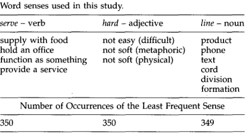
Table 1

Word senses used in this study.

serve - verb hard - adjective line - noun

supply with food not easy (difficult) product hold an office not soft (metaphoric) phone function as something not soft (physical) text

provide a service cord

division formation Number of Occurrences of the Least Frequent Sense

350 350 349

' p r o d u c t ' sense of l i n e from the W a l l S t r e e t J o u r n a l , t h e n w e could h a v e i m p r o v e d u p o n

the results p r e s e n t e d in the next section b y simply always guessing 'product'. 4. N e u r a l - N e t w o r k - b a s e d S e n s e D i s a m b i g u a t i o n

This section s u m m a r i z e s a series of e x p e r i m e n t s that tests w h e t h e r neural n e t w o r k s can extract sufficient i n f o r m a t i o n from sample usages to accurately resolve w o r d senses. We choose neural n e t w o r k s as the learning m e t h o d for this s t u d y because o u r p r e v i o u s w o r k has s h o w n neural n e t w o r k s to be m o r e effective than several other m e t h o d s of sense disambiguation (Leacock, Towell, Voorhees 1996). Moreover, there is a m p l e empirical evidence w h i c h indicates that neural n e t w o r k s are at least as effective as other learning systems on most p r o b l e m s (Shavlik, Mooney, and Towell 1991; Atlas et al. 1989). The major d r a w b a c k to neural n e t w o r k s is that they m a y require a large a m o u n t of training time. For o u r purposes, training time is not an issue, since it m a y be d o n e off-line. H o w e v e r , the time required to classify an example is significant. Because of its complexity, o u r a p p r o a c h will almost certainly be slower than m e t h o d s such as decision trees. Still, the time to classify an example will most likely be d o m i n a t e d b y the time required to t r a n s f o r m an example into the a p p r o p r i a t e f o r m a t for i n p u t to the classifier. This time will be r o u g h l y u n i f o r m across classification strategies, so the difference in the s p e e d of the various classification m e t h o d s themselves s h o u l d be unnoticable.

[image:5.468.34.285.75.211.2]

(6)

number of labeled training examples plus a larger number of unlabeled examples. Experimental results demonstrate that SULU consistently and significantly improves classification accuracy when there are few labeled training examples.

4.1 Asymptotic Accuracy

All of the neural networks used here are strictly feed-forward (Rumelhart, Hinton, and Williams

1986). By

this, we mean that there is a set of

input units

that receive activation only from outside the network. The input units pass their activation on to

hidden units

via weighted

links.

The hidden units, in turn, pass information on to either additional hidden units or to

output units.

There are no recurrent links; that is, the activation sent by a unit can never, even through a series of intermediaries, be an input to that unit.

Units that are not input units receive activation only via links. The non-input 1 where x is the sum of the incoming activations units compute the function y - l+e-x

weighted by the links and y is the output activation. (The translation of words into numbers so that this formula can be applied to word sense disambiguation is described in the following paragraphs.) This nonlinear function has the effect of squashing the input into the range [0... 1]. Output units give the answer for our networks. Finally, the activation of the output units is normalized so that their sum is 1.0.

In all of the experiments reported below, the weights on all the links are initially set to random numbers taken from a uniform distribution over [ - 0 . 5 . . . 0.5]. The networks are then trained using gradient descent algorithms (e.g., backpropagation [Rumelhart, Hinton, and Williams 1986]) so that the activation of the output units is similar to some desired pattern. Networks are trained until either each example has been presented to the network 100 times or at least 99.5% of the training patterns are close enough to the desired pattern that they would be considered correct. (The meaning of "correct" will vary in our experiments, it will be clearly defined in each experiment.) In practice, the second stopping criterion always obtained.

The networks used in most of this work have a very simple structure: one output trait per sense, one input unit per token (the meaning of "token" differs between local and topical networks as described below), and no hidden units. For both local and topical encodings, we tested m a n y hidden unit structures, including ones with m a n y layers and ones with large numbers of hidden units in a single layer. However, with one exception described below, a structure with no hidden units consistently yields the best results. Input units are completely connected to the output units; that is, every input unit is linked to every output unit. During training, the activation of the output trait corresponding to the correct sense has a target value of 1.0, the other outputs have a target value of 0.0. During testing, the sense reported by the network is the output unit with the largest activation. An example is considered to be classified correctly if the sense reported by the network is the same as the tagged sense.

(7)

8 gi

[image:7.468.36.327.53.161.2]

N 8

Figure 1

Oc. -

~ ~ O O ~ = ~ ~ ¢ ~ O H a r d - local

0 ~ , , , ~ ~ ~ H a r d - t o p i c a l

0 ~O ~ ' ° " ~ ~ L i n e - t o p i c a l - o - - o L i n e - local • .' ' e ~ ' " S e r e - t o p i c a l 0 - O - S e r v e - local

SO0 I000 1500 2000

Number of Examples

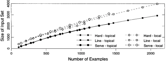
The effect of increasing example size on the number of input units needed for encoding. For each of our three data sets and each encoding method, this figure shows the number of input units required to encode the examples. Except for the endpoints, which use the entire example set, each point is the average of 11 random selections from the population of examples.

To e n c o d e a n e x a m p l e for a n e t w o r k that extracts local context, each t o k e n ( w o r d or p u n c t u a t i o n ) is p r e p e n d e d w i t h its p o s i t i o n relative to the target a d d i n g p a d d i n g as necessary. For e x a m p l e , g i v e n the sentence "John serves loyally.", the target serves,

a n d a desire to u s e three t o k e n s on either side of the target, the i n p u t to the n e t w o r k is [-3zzz -2zzz -1John 0serves 1loyally 2. 3zzz] w h e r e " z z z " is a d d e d as a b l a n k as n e e d e d . N e t w o r k s contain i n p u t units r e p r e s e n t i n g e v e r y resulting string w i t h i n three of the target w o r d in the set of labeled training e x a m p l e s . N o t e that this implies that there will be w o r d s in positions in the test set that are n o t m a t c h e d in the training set. So, while training e x a m p l e s will h a v e exactly s e v e n i n p u t units w i t h a v a l u e of 1.0, testing e x a m p l e s will h a v e at m o s t s e v e n i n p u t units w i t h a v a l u e of 1.0. The w i n d o w w e use is slightly w i d e r t h a n a w i n d o w of t w o w o r d s on either side that e x p e r i m e n t s w i t h h u m a n s s u g g e s t is sufficient ( C h o u e k a a n d L u s i g n a n 1985). The h u m a n s t u d y c o u n t e d o n l y w o r d s , w h e r e a s w e c o u n t b o t h w o r d s a n d p u n c t u a t i o n . O u r n e t w o r k s are significantly less accurate u s i n g w i n d o w s smaller t h a n three t o k e n s on either side. O n the other h a n d , w i d e r w i n d o w s are slightly, b u t not statistically significantly, m o r e accurate.

Figure 1 s h o w s that the topical a n d local e n c o d i n g m e t h o d s result in large i n p u t sets. For e x a m p l e , w h e n the entire p o p u l a t i o n of line e x a m p l e s is used, the local en- c o d i n g w o u l d require 3,973 i n p u t units a n d the topical e n c o d i n g w o u l d require 2,924 inputs. Fortunately, this figure s h o w s that the rate of increase in the size of the in- p u t set steadily decreases as the size of the i n p u t set increases. Fitting each of the lines in this figure against e x p o n e n t i a l functions indicates that n o n e of these d a t a sets w o u l d g r o w to require m o r e t h a n 9,000 i n p u t s units. While this is certainly large, it is tolerable.

We i n v e s t i g a t e d m a n y w a y s of c o m b i n i n g the o u t p u t of the topical a n d local n e t w o r k s . We r e p o r t results for a m e t h o d that takes the m a x i m u m of the s u m of the o u t p u t units. 2 For e x a m p l e , s u p p o s e that a local n e t w o r k for d i s a m b i g u a t i n g the three senses of hard h a s o u t p u t s of (0.4 0.5 0.1) a n d a topical n e t w o r k h a s o u t p u t s of (0.4

2 Among the many alternatives we investigated for merging the local and topical networks, only one yields slightly better results. It is based upon Wolpert's stacked generalization (Wolpert 1992). In this technique, the outputs from the topical and local networks are passed into another network whose function is simply to learn how to combine the outputs. When the input to the combining network is the concatenation of the inputs and the outputs of both the local and topical networks, the combining network often outperforms our summing method. However, the improvement is usually not

(8)

0.0 0.6). Then the local information would suggest the second sense, while the topical information would suggest the third sense. The summing strategy yields (0.8 0.5 0.7), so the combined classifier would select the first sense.

The only approach we have found that consistently, and statistically significantly, outperforms the strategy described above is based upon error-correcting output encoding (Kong and Dietterich 1995). The idea of error-correcting codes is to learn all possible dichotomies of the set of classifications. For example, given a problem with four classes, A, B, C, and D, learn to distinguish A and B from C and D; A from B, C, and D; etc. The major problem with this method is that it can be computationally intensive when there are m a n y output classes because there are 2 s-1 - 1 dichotomies for S output classes. We implemented error-correcting output codes by independently training a network with one output unit and 10 hidden units to learn each dichotomy. 4.1.1

Testing Methodology.

To estimate the accuracy of our disambiguation methods, we built learning curves using several values of N in N-fold cross-validation. In cross- validation, the data set is randomly divided into N equal parts, then N - 1 parts are used for training and the remaining part is held aside to assess generalization. 3 As a result, each example is used for training N - 1 times and once to assess generalization. A drawback of N-fold cross-validation is that it cannot test small portions of the data. So, for points on the learning curves that use less than 50% of the training data, we invert the cross validation procedure, using one of the N parts for training and the remaining N - 1 parts to assess generalization. For example, if there are 100 labeled examples, each iteration of 10-fold cross-validation would use 90 examples for training and the remaining 10 for testing. When complete, each example would be used for training exactly nine times and exactly once for testing. By contrast, in inverted 10-fold cross-validation, each example is used exactly once for training and exactly nine times for testing.

4.1.2

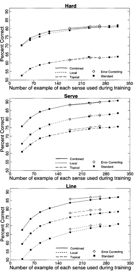
Results and Discussion.

The learning curves are shown in Figure 2. Each point in the figure represents an average over 11 cross-validation trials. Thus, the point for 75% of the training set, which corresponds to 4-fold cross-validation, requires training 44 networks. The confusion matrices in Tables 2 to 4 give the complete data for the largest training sets of the "standard" curves in Figure 2. Rows in the table represent the correct answer, and columns represent the answer selected by the classifier. "Total" gives the number of times the classifier selects the given sense. "Precision" is the percentage of that total that is correct. In contrast, "Percent Correct" gives the accuracy of the classifier over the set of hand-tagged examples of the given sense.

Figure 2 shows that, for line and serve, the combined classifier is considerably superior to either the local or topical classifier at all training-set sizes. At the largest training-set size, the combined classifier is superior with at least 99.5% confidence according to a one-tailed paired-sample t-test. There is no advantage for the combined classifier for hard. In fact, at the largest training-set size, the local classifier slightly outperforms the combined classifier. The difference, while small, is statistically significant with 97.5% confidence according to a one-tailed paired-sample t-test.

An obvious reason, as can be seen in Figure 2, for w h y the combined representation fails to improve classification effectiveness for hard is that the topical classifier

(9)

Towell and Voorhees Disambiguating Highly Ambiguous Words

E R

Hard

=o

( E r - -

2 ~ a-=o

i l l ~ - - Combined

O Error Correcting

i " / . . . Local

• Standard

- - - - - - Topical

7b 14o 2~o 2~o

Number of example of each sense used during training Serve

. , - ' o t ~ c o

. ~ . . . l i > ~ - - Q - - ~ - t - , ~

"" _ ~ V ~ ~ ' ~ ~ - ~ -

. m - - - t

/ =" .,Jr"

/

Combined

. . . L o c a l 0 Error Correcting

• Standard

- - - - - - Topical

~'0 1,i0 2to 2~o

Number of example of each sense used during training

Line

• / . / o---T.Y_--= . . . .

OLO I m - - -

~ ¢ . O J " ' ' "

/ / . I - - - ' ' "

~ .~ •

I " - - Combined

" - . . . L o c a l O Error Correcting

• Standard

- - - - - - Topical

710 1 4 0 2 1 0 a~0 ) 0

Number of example of each sense used during training

Figure 2

Learning curves for classifiers that use local context only (Local), topical context only (Topical), and a combination of local and topical contexts (Combined) for hard, serve, and line. Each point in each curve represents an average over 11 repetitions of N-fold cross-validation. The points on each of these curves represent 10-, 6-, 4-, 3-, and 2-fold cross-validation and 3-, 4-, and 6-fold inverted cross-validation. Error-correcting codes have results at only 2-, 3-, and 4-fold cross-validation (i.e, 50%, 66%, and 75% of the training data.)

is m u c h w o r s e than the local classifier. While the differences in accuracy b e t w e e n the topical and local classifiers are statistically significant w i t h at least 99.5% c o n f i d e n c e according to a one-tailed p a i r e d - s a m p l e t-test o n all three senses, the accuracies are m o r e similar for b o t h serve a n d line than t h e y are for hard. This o b v i o u s difference in accuracy is o n l y part o f the reason w h y the c o m b i n e d classifier is less effective for hard.

[image:9.468.38.259.45.490.2]

(10)

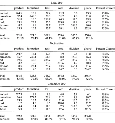
Table 2

Average confusion matrices for hard over 11 runs of 10-fold cross validation. Rows in the table represent the correct answer, columns represent the answer given by the classifier. So, in the local table, 22.1 is the average number of times that the classifier selected the 'physical' sense when the correct sense was the 'difficult' sense. There are 350 examples of each class.

Local-hard

difficult metaphoric physical Percent Correct

difficult 301.5 26.5 22.1 86.1%

metaphoric 23.2 256.4 70.5 73.2%

physical 13.9 33.6 302.5 86.4%

Total 338.5 316.5 395.0

Precision 89.0% 81.0% 76.6%

Topical-hard

difficult 210.6 98.0 41.4 60.2%

metaphoric 114.8 203.6 31.5 58.2%

physical 56.1 40.1 253.8 72.5%

Total 381.5 341.7 326.7

Precision 55.2% 59.6% 77.7%

Combined-hard

difficult 299.0 35.7 15.3 85.4%

metaphoric 62.3 247.8 39.9 70.8%

physical 20.1 24.6 305.3 87.2%

Total 381.4 308.2 360.5

Precision 78.4% 80.4% 84.7%

are m o r e h i g h l y correlated for hard t h a n for either line or serve. The a v e r a g e correlation of correct a n d incorrect a n s w e r s for local a n d topical classifiers of hard is 0.14 while the a v e r a g e correlations for line a n d serve, respectively, are 0.07 a n d - 0 . 0 2 . M a n y efforts at u s i n g e n s e m b l e s of classifiers h a v e r e p o r t e d that to get significant i m p r o v e m e n t s , the m e m b e r s of the e n s e m b l e s h o u l d be as u n c o r r e l a t e d as possible ( P a r a m a n t o , M u n r o , a n d D o y l e 1996). G i v e n the correlation b e t w e e n the local a n d topical classifiers for

[image:10.468.48.326.135.454.2]

(11)

Table 3

Average confusion matrices for serve over 11 runs of 10-fold cross validation.

Rows in the table represent the correct answer, columns represent the answer given by the classifier. So, in the local table, 6.7 is the average number of times that the classifier selected the 'food' sense when the correct sense was the 'function as' sense. There are 350 examples of each class.

Local-serve

function as service food office Percent Correct

function as 293.7 22.9 6.7 26.6 83.9%

service 5.8 312.9 26.1 5.2 89.4%

food 5.7 43.4 283.4 17.5 81.0%

office 41.5 14.1 18.3 276.1 78.9%

Total 346.8 393.3 334.5 325.5

Precision 84.7% 79.6% 84.7% 84.8%

Topical-serve

function as 218.0 51.2 30.6 50.2 62.3%

service 50.0 261.1 5.8 33.1 74.6%

food 22.2 4.3 308.2 15.4 88.1%

office 40.1 29.9 10.8 269.2 76.9%

Total 330.3 346.5 355.5 367.8

Precision 66.0% 75.4% 86.7% 73.2%

Combined-serve

function as 298.4 23.4 5.8 22.5 85.2%

service 14.0 321.0 5.7 9.3 91.7%

food 2.5 7.5 333.8 6.1 95.4%

office 22.7 8.7 3.7 314.8 89.9%

Total 337.6 360.6 349.1 352.6

Precision 88.4% 89.0% 95.6% 89.3%

the ' p r o v i d e f o o d ' sense w h e n the correct sense is either ' f u n c t i o n as' (5.8) or ' p r o v i d e a service' (5.7).

This pattern of offsetting errors is repeated on all b u t one of the senses of line

a n d serve. W h e r e v e r it occurs, the c o m b i n e d classifier is superior to b o t h the local a n d topical classifiers. By contrast, errors for the local a n d topical classifiers of hard

[image:11.468.39.352.124.478.2]

(12)

Table 4

Average confusion matrices for line over 11 runs of 10-fold cross validation. Rows in the table

represent the correct answer, columns represent the answer given by the classifier. So, in the local table, 16.7 is the average number of times that the classifier selected the 'formation' sense when the correct sense was the 'product' sense. There are 349 examples of each class.

Local-line

product formation text cord division phone Percent Correct

product 264.5 16.7 27.4 21.3 5.6 13.5 75.8%

formation 32.4 248.0 20.8 31.2 4.8 11.8 71.1%

text 31.8 16.5 218.7 44.5 17.5 19.9 62.7%

cord 19.1 23.2 35.5 215.8 12.9 42.5 61.8%

division 8.2 9.8 21.7 12.7 286.5 10.0 82.1%

phone 15.9 10.2 33.7 28.1 8.2 252.9 72.5%

Total 371.8 324.5 357.9 353.6 335.5 350.6

Precision 71.1% 76.4% 61.1% 61.0% 85.4% 72.1%

Topical-line

product 294.7 13.1 17.8 1.9 9.6 11.8 84.4%

formation 16.7 236.1 51.5 8.3 20.0 16.4 67.6%

text 19.5 40.8 238.7 4.7 33.7 11.5 68.4%

cord 3.2 6.0 13.0 311.6 4.9 10.3 89.3%

division 8.5 23.4 28.7 13.5 263.4 11.6 75.5%

phone 9.0 9.3 16.1 14.2 6.3 294.2 84.3%

Total 351.6 328.6 365.9 354.2 337.9 355.7

Precision 83.8% 71.8% 65.2% 88.0% 77.9% 82.7%

Combined-line

product 317.3 8.1 9.8 4.8 2.9 6.1 90.9%

formation 16.6 279.3 26.4 11.2 4.8 10.7 80.0%

text 13.9 16.2 280.4 11.0 16.5 11.1 80.3%

cord 1.7 4.5 8.6 318.0 4.5 11.7 91.1%

division 4.4 7.4 11.5 7.5 312.5 5.7 89.6%

phone 5.3 5.6 11.5 12.6 2.5 311.5 89.2%

Total 359.2 321.0 348.1 365.2 343.7 356.8

Precision 88.3% 87.0% 80.5% 87.1% 90.9% 87.3%

' d i f f i c u l t ' a n d ' m e t a p h o r i c ' s e n s e s of hard m o r e t h a n offset the e r r o r s e l i m i n a t e d b y the ' p h y s i c a l ' sense. Therefore, t h e local classifier for hard is m o r e a c c u r a t e t h a n the c o m b i n e d classifier.

The t o p i c a l classifier o u t p e r f o r m s the local classifier for the n o u n line (Figure 2). C o n v e r s e l y , the local classifier o u t p e r f o r m s the t o p i c a l classifier for the v e r b serve

[image:12.468.52.432.129.535.2]

(13)

the topical representation should add only confusion. Hence, one would expect to see the local classifier outperforming the topical classifier for all adjectives. Similarly, some verb senses are determined largely by their direct object. For example, the 'provide a service' sense of serve almost always has a thing as a direct object, while the 'function as' sense of serve almost always has a person. The added information in the topical encoding may obscure this difference, thereby adding to the difficulty of correctly disambiguating these senses. So, we would not be surprised to see the advantage of local representations over topical representations continue on other verbs and adjectives.

Many techniques for using local context explicitly use diagnostic phrases, such as wait in line, for the formation sense of line. In previous work, we took exactly this approach and showed that diagnostic phrases could be used to improve the accuracy of a topical classifier (Leacock, Towell, and Voorhees 1996). Our neural network for local disambiguation differs considerably from this approach. Specifically, it is unable to learn more than one diagnostic phrase per sense because it lacks hidden units. In fact, the network does not learn a single diagnostic phrase. Instead, it learns that certain words in certain positions are indicative of certain senses. While this might appear to be a significant handicap, we have been unable to train a network that is capable of learning phrases so that it outperforms our networks. In addition, while they lack the ability to learn phrases, our local classifiers are, nonetheless, quite effective at determining the correct sense. It is our belief that hidden units would be useful for learning local context given a sufficient amount of training data. However, there are currently far more free parameters in our networks than there are examples to constrain those parameters. Until there are more constraints, we do not believe that hidden units will be useful for sense disambiguation.

Finally, it is interesting to note that not all senses are equally easy, and that different classifiers find different senses easier than others. For example, in Table 2 the most difficult sense of hard for the local classifier is the 'physical' sense, but this is the easiest sense for both the topical and combined classifiers. On the other hand, some senses are just difficult. The 'text' sense of line (Table 4) is among the hardest for all classifiers. We believe that the 'text' sense is difficult because it often contains quoted material which m a y distract from the meaning of line. However, the quoted material is often too far away from the target word for the quotation marks to be seen in the local window. As a result, the topical classifier is confused by distracting material and the local classifier does not see the most salient feature.

4.2 Senses Missing from Data

The results in the previous section suggest that, given a sufficiently large number of labeled examples, it is possible to combine topical and local representations into an effective sense classifier. Those results, however, assume that the labeled examples include all possible senses of the word to be disambiguated. Senses not included in the training set will be misclassified because the procedure assigns a sense to every example. In this section, we allow the system to respond do not know to address the issue of senses not seen during training.

(14)

Table 5

The chance rate of correct rejection rate for each of the target words. (All numbers are percentages.)

Target Word Overall Resulting from Resulting from Unknown Senses Errors on Known Senses

hard 47 33 14

serve 32 25 7

line 25 17 8

is greater t h a n a threshold. W h e n the m a x i m u m activation is b e l o w the threshold, the n e t w o r k ' s response is do not know.

The logic u n d e r l y i n g this modification is that the activation of the o u t p u t unit c o r r e s p o n d i n g to the correct a n s w e r tends to be close to 1.0 w h e n the instance to be classified is similar to a training example. Hence, instances of senses seen d u r i n g training s h o u l d h a v e an o u t p u t unit w h o s e activation is close to 1.0 (assuming that the training examples a d e q u a t e l y represent the set of possibilities). On the other h a n d , instances of senses not seen d u r i n g training are unlikely to be similar to a n y training example. So, t h e y are unlikely to generate an activation that is close to 1.0.

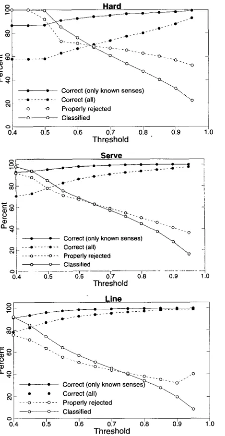
4.2.1 Testing Methodology. We use a l e a v e - o n e - c a t e g o r y - o u t p r o c e d u r e to test o u r h y p o t h e s i s that w e can detect u n k n o w n senses b y screening for examples that h a v e a low m a x i m u m o u t p u t activation. O u r p r o c e d u r e is as follows: n e t w o r k s are trained using 90% of the examples of S - 1 senses w h e n there are S senses for a target w o r d . The trained n e t w o r k is then tested using the u n u s e d 10% of the S - 1 classes seen d u r i n g training and 10 percent of the examples of the class not seen d u r i n g training (selected r a n d o m l y ) . In addition, d u r i n g testing the n e t w o r k is g i v e n a threshold v a l u e to d e t e r m i n e w h e t h e r or n o t to label the example. Figure 3 s h o w s the effect of v a r y i n g the threshold f r o m 0.4 to 1.0 (values b e l o w 0.4 w e r e tried b u t h a d no effect) using the c o m b i n e d classifier. The l e a v e - o n e - c a t e g o r y - o u t p r o c e d u r e was r e p e a t e d 11 times for each sense.

4.2.2 Results and Discussion. The g r a p h s in Figure 3 s h o w that the slight modification of the classifier has the h y p o t h e s i z e d effect. N o t surprisingly, the n u m b e r of examples classified always decreases as the threshold increases. Also e x p e c t e d is that the percentage of correctly rejected examples falls as the threshold i n c r e a s e s - - i n c r e a s i n g the threshold naturally catches m o r e examples that s h o u l d be accepted. (A rejected ex- a m p l e is one for w h i c h the classifier r e s p o n d s do not know.) The up-tick in the p r o p e r rejection rate at high thresholds for line is not significant. Of m o r e interest is that the classifier is always significantly better than chance at correctly rejecting examples. The chance rate of correct rejection is s h o w n in Table 5. Thus, the modification allows the classifier to identify senses that d o n o t a p p e a r in the training set.

(15)

°~

o

~ o ('- (DI Q)

o

a_o

Hard

~ ~°--.x 3 ~°--. x 3

= ; Correct (only k n o w ~

- - - . . . . • - Correct (all) o .o Properly rejected

- - - ~ o n - Classified

~.4 01s 016 017 018 019 1.0

Threshold

Serve

g

J

_I

.j

; : Correct (only kno senses)

o ---e- - ~ - - Correct (all) " ~

- - -o . . . . -o-- Properly rejected

- ~ o ~ Classified

0.4 0.5 0.6 0.7 0'3 0.9 1.0

Threshold

Line

Qo

.... ~--i

i _ _ _ i _ _ i i i i ~ e ~ r i ! i ! ; : ~ : : w n s e n s ~

Classified

% 0'.s 016 017 018 0!9 t.o

Threshold

[image:15.468.42.268.48.485.2]

§3

Figure 3

The effect of omitting one sense from the training set. In each figure, the X-axis represents the level of a threshold. If the maximum output activation is below the threshold then the

network responds do not know. "Correct (only known senses)" gives the accuracy of the

combined classifier on senses seen during training. "Correct (all)" gives the accuracy over all examples. "Properly rejected" is the percentage of all examples for which the classifier

responds do not know that are either in a novel sense or would have been misclassified. Finally,

"Classified" gives the percentage of the data for which the classifier assigns a sense.

4.3 Using Small Amounts of Labeled Data

(16)

RANDOM(min,max):

r e t u r n a u n i f o r m l y d i s t r i b u t e d r a n d o m integer b e t w e e n m i n and max, i n c l u s i v e

MAIN(B,M):

/* B - in [0...I00], controls the rate of e x a m p l e synthesis */

/* M - controls n e i g h b o r h o o d size d u r i n g synthesis */

Let: E /* a set of l a b e l e d e x a m p l e s */

U /* a set of u n l a b e l e d e x a m p l e s */

N /* an a p p r o p r i a t e n e u r a l n e t w o r k */

Repeat P e r m u t e E For each e in E

if random(O,lO0) > B t h e n

e <- S Y N T H E S I Z E (e, E, U, r a n d o m (2, M) ) T R A I N N u s i n g e

U n t i l a s t o p p i n g c r i t e r i o n is r e a c h e d

S Y N T H E S I Z E ( e , E , U , m ) :

Let: C /* will h o l d a c o l l e c t i o n of e x a m p l e s */

For i f r o m I to m

c <- ith n e a r e s t n e i g h b o r of e in E u n i o n U

if.((c is labeled) and (label of c not equal to label of e)) t h e n STOP if c is not l a b e l e d

cc <- n e a r e s t n e i g h b o r of c in E

if label of cc not equal to label of e t h e n STOP add c to C

[image:16.468.44.384.77.351.2]

r e t u r n an e x a m p l e whose input is the c e n t r o i d of the inputs of the e x a m p l e s in C and has the class label of e.

Figure 4

Pseudocodefor SULU.

examples barely sufficient to get them started on the learning curve.

While labeled examples will likely always be rare, unlabeled text is already available in huge quantities. Theoretical results (Castelli and Cover 1995) suggest that it should be possible to use both labeled and unlabeled examples to produce a classifier that is more accurate than one based on only labeled examples. We describe an algorithm, SULU (Supervised learning Using Labeled and Unlabeled examples), that uses both labeled and unlabeled examples and provide empirical evidence of the algorithm's effectiveness (Towell 1996).

4.3.1 The SULU Algorithm. SULU uses standard neural-network supervised training techniques except that it may replace a labeled example with a synthetic example. A synthetic example is a point constructed from the nearest neighbors of a labeled example. The criterion to stop training in SULU is also slightly modified to require that the network correctly classify almost every labeled example and a majority of the synthetic examples. For instance, the experiments reported below generate synthetic examples 50% of the time; the stopping criterion requires that 80% of the examples seen in a single pass through the training set (an epoch) are classified correctly.

(17)

to get information about the local variance around known points, this criterion guar- antees locality. Second, the next closest example to the seed is a labeled example with a different label: this criterion prevents the inclusion of obviously incorrect information in synthetic examples. Third, the next closest example to the seed is an unlabeled example and the closest labeled example to that unlabeled example has a different label from the seed: this criterion is intended to detect borders between classification areas in example space.

4.3.2

Testing Methodology.

The following methodology is used to test SULU on each data set. First, the data are split into three sets, 25% is set aside to be used for assessing generalization, 50% is stripped of sense labels, and the remaining 25% is used for training. To create learning curves, the training set is further subdivided into sets of 5%, 10%, 15%, 20%, and 25% of the data, such that smaller sets are always subsets of larger sets. Then, a single neural network (of the structure described in Section 4.1) is created and copied 25 times. At each training-set size, a new copy of the network is trained under each of the following conditions: (1) using SULU, (2) using SULU but supplying only the labeled training examples to s y n t h e s i z e , (3) standard network training, (4) using a re-implementation of an algorithm proposed by Yarowsky (1995), and (5) using standard network training but with all training examples labeled to establish an upper bound. This procedure is repeated 11 times to average out the effects of example selection and network initialization.

Yarowsky's algorithm expands the region of known, labeled examples out from a small set of hand-labeled seed collocations. Our instantiation of Yarowsky's algorithm differs from the original in three ways. First, we use neural networks whereas Yarowsky uses decision lists. This difference is almost certainly not significant; in describing his algorithm, Yarowsky notes that a neural network could be used in place of decision lists. Second, we omit the application of the one-sense-per-discourse heuristic, as our examples are not part of a larger discourse. This heuristic could be equally applied to SULU, so eliminating this heuristic from Yarowsky's algorithm places the algorithms on an equal base. Finally, we randomly pick the initially labeled contexts. The effect of this difference could be significant. However, this difference would affect our system as well as Yarowsky's, so it should not invalidate our comparison.

When SULU is used, synthetic examples replace labeled examples 50% of the time. Networks using the full SULU (condition i above) are trained until 80% of the examples in a single epoch are correctly classified. All other networks are trained until at least 99.5% of the examples are correctly classified.

4.3.3

Results and Discussion.

The graphs in Figure 5 show the efficacy of the combined classifier for each algorithm on each of our three target words. SULU always re- suits in a statistically significant improvement over the standard neural network with at least 97.5% confidence (according to a one-tailed paired-sample t-test). Interestingly, SULU'S improvement is consistently between ¼ and ½ of that achieved by labeling the unlabeled examples. This result contrasts with Castelli and Cover's (1995) analysis that suggests that labeled examples are exponentially more valuable than unlabeled examples.

SULU is consistently and significantly superior to our version of Yarowsky's algorithm when there are few labeled examples. As the number of labeled examples increases the advantage of SULU decreases. At the largest training-set sizes tested, the two systems are roughly equally effective.

(18)

Computational Linguistics Volume 24, Number 1

H a r d

standard with 700 labeled

c~ _ ~ SULU with 700 unlabeled

- - - Yarowsky with 700 unlabeled

~ 0 " _ ~ - - - SULU with 0 unlabeled

EE eq ~ + Statistically superior to SULU

" ~ ~ ~"O'---.- 0 Statistically inferior to SULU

•

: "~" "'~-.I-.-~-- . . . . ~ . . . . +

. . . . . . ....... . . . o

o

"rs'0 160 lg0 260 2g0

Size of labeled training set

S e r v e

-§

O_

C ,..r~ ¢J

~ o

O . 4?

o

0

~ o

O .

" ~ L O

~ o

O .

0

standard with 700 labeled

SULU with 700 unlabeled

+~

. . . Yarowsky with 700 unlabeled

SULU with 0 unlabeled

• ~ ~ - + Statistically superior to SULU - ~ 0 Statistically inferior to SULU

0 " "

160 1~0 200 2g0 360

350

S i z e of labeled training set

L i n e

- - - - standard with 1046 labeled

SULU with 1046 unlabeled

- Yarowsky with 1046 unlabeled

- - - SULU with 0 unlabeled

+ Statistically superior to SULU

~ ~ 0 Statistically inferior to SULU

. ~ 0 -

-8t

. .. . . 8 - 7 - - ~ - - ~ - 8 . . . ~ ...

)0 1 SO 2 0 0 2 g O 3 6 0 3 g O 4 6 0 4 g O 5 0 0

Size of labeled training set

Figure 5

The effect of five training procedures on the target words. In each of the above graphs, the effect of standard neural learning has been subtracted from all results to suppress the increase in accuracy that results simply from an increase in the number of labeled training examples. Observations marked by a "o" or a "+", respectively, indicate that the point is statistically significantly inferior or superior to a network trained using SULU.

h y p o t h e s i s is incorrect. A s s h o w n in Figure 5, w h e n SULU is g i v e n n o u n l a b e l e d ex- a m p l e s it is consistently a n d significantly inferior to SULU w h e n it is g i v e n a large n u m b e r of u n l a b e l e d e x a m p l e s . In addition, s u g u w i t h n o u n l a b e l e d e x a m p l e s is c o n - sistently, a l t h o u g h n o t a l w a y s significantly, inferior to a standard neural n e t w o r k (data n o t s h o w n ) .

[image:18.468.45.272.48.494.2]

(19)

generalization between sucu and a network trained using data in which the unlabeled examples provided to SULU have labels (condition 5 above). On every data set, the gain from labeling the examples is statistically significant. The accuracy of a network trained with all labeled examples is an upper bound for SULU, and one that is likely not reachable. However, the distance between this upper bound and SULU'S current performance indicates that there is room for improvement.

5. C o n c l u s i o n

The goal of our sense disambiguation work is to develop a classifier that allows information retrieval systems to exploit the semantics encoded in lexical systems such as WordNet to improve retrieval performance. To be useful in that environment, the classifier must be effective at distinguishing the senses included in the lexicon and efficient enough to use during query processing. As a first step towards this goal, we have developed a classifier that is able to select the sense of a single highly ambiguous word given the two-sentence context in which the word appears.

We tested our sense disambiguation approach on three highly polysemous words: six noun senses of line, four verb senses of serve, and three adjective senses of hard.

The performance of our disambiguator on these three tasks was quite good; it has an average accuracy of 87%, 90%, and 81%, respectively, when it is forced to label all test examples. The labeling accuracy of our method can be further improved by allowing it to respond do not know on a small percentage of the test examples.

While our current plan is to resolve the sense of each query term independently, some modifications to the current classifier may provide for the simultaneous classification of multiple polysemous words in a single context. By changing from backpropagation to the EM algorithm (Dempster, Laird, and Rubin 1977), we can jointly refine poor guesses of the senses of the words with feedback from prior iterations.

Our desire to use the sense classifier as part of a query-processing step influenced the types of classifiers we considered. The error-correcting codes networks discussed in Section 4.1 offer the potential for slightly higher accuracy rates than our simple sum combination, but at a significantly higher cost in time and space. Hence, we concentrated our effort on a simple scheme for combining local and topical neural networks using a sum of the output activations. Using this method, the expense of using the classifier would be dominated by the time and space requirements needed to break the query into tokens and to map those tokens to the correct input units of the various networks.

(20)

References

Atlas, Les, Ronald Cole, Jerome Connor, Mohamed E1-Sharkawi, Robert J. Marks II, Yeshwant Muthusamy, and Etienne Barnard. 1989. Performance comparisons between backpropagation networks and classification trees on three real-world applications. In Advances in Neural Information Processing Systems, volume 2, pages 622-629, Denver, CO. Morgan Kaufmann.

Black, Ezra W. 1988. An experiment in computational discrimination of English word senses. IBM Journal of Research and Development, 32(2):185-194.

Brill, Eric. 1992. A simple rule-based part of speech tagger. In Proceedings of the Third Conference on Applied Computational Linguistics (ACL).

Castelli, Vittorio and Thomas M. Cover. 1995. The relative value of labeled and unlabeled samples in pattern recognition with an unknown mixing parameter. Technical Report 86, Stanford University, Department of Statistics.

Choueka, Yaacov and Serge Lusignan. 1985. Disambiguation by short contexts. Computers and the Humanities, 19:147-157. Dempster, A. P., N. M. Laird, and D. B.

Rubin. 1977. Maximum likelihood from incomplete data via the EM algorithm. Journal of the Royal Statistical Society B, 39:1-38.

Gale, William, Kenneth W. Church, and David Yarowsky. 1992. A method for disambiguating word senses in a large corpus. Computers and the Humanities, 26. Harman, Donna K. 1993. The first Text

REtrieval Conference (TREC-1), Rockville, MD, U.S.A, 4-6 November, 1992.

Information Processing and Management, 29(4):411-~414.

Hearst, Marti A. 1991. Noun homograph disambiguation using local context in large text corpora. In Proceedings of the Seventh Annual Conference of the UW Centre for the New OED and Text Research: Using

Corpora, pages 1-22, Oxford.

Kong, Eun Bae and Thomas G. Dietterich. 1995. Error-correcting output coding corrects bias and variance. In Proceedings of the Twelfth International Conference on Machine Learning, pages 313-321, Morgan Kaufmann.

Krovetz, Robert and W. Bruce Croft. 1992. Lexical ambiguity in information retrieval. ACM Transactions on Information Systems, 10(2):115-141.

Leacock, Claudia, Geoffrey Towell, and

Ellen M. Voorhees. 1993. On 'line' learning, unpublished.

Leacock, Claudia, Geoffrey Towell, and Ellen M. Voorhees. 1996. Towards building, contextual representations of word senses using statistical models. In B. Boguraev and J. Pustejovsky, editors, Corpus Processing for Lexical Acquisition. MIT Press, pages 97-113. Originally appeared in Proceedings of SIGLEX Workshop: Acquisition of Lexical Knowledge from Text, 1993.

Miller, George. 1990. Special Issue, WordNet: An on-line lexical database. International Journal of Lexicography, 3(4). Miller, George A. and Walter G. Charles.

1991. Contextual correlates of semantic similarity. Language and Cognitive Processes, 6(1).

Paramanto, Bambang, Paul W. Munro, and Howard R. Doyle. 1996. Improving committee diagnosis with resampling techniques. In D. Touretzky, M. Mozer, and M. Hasselmo, editors, Advances in Neural Information Processing Systems, volume 8, Denver, CO. MIT Press. Quinlan, J. Ross. 1992. C4.5. Morgan

Kaufmann, Santa Cruz, CA.

Rumelhart, David, Geoffrey Hinton, and Ronald Williams. 1986. Learning internal representations by error propagation. In David Rumelhart and James McClelland, editors, Parallel Distributed Processing: Explorations in the Microstructure of Cognition. Volume 1: Foundations. MIT Press, Cambridge, MA, pages 318-363. Salton, Gerald and Michael E. Lesk. 1971.

Computer evaluation of indexing and text processing. In Gerard Salton, editor, The SMART Retrieval System: Experiments in Automatic Document Processing.

Prentice-Hall, Inc., Englewood Cliffs, NJ, pages 143-180.

Salton, Gerald, A. Wong, and C. S. Yang. 1975. A vector space model for automatic indexing. Communications of the ACM, 18(11):613-620.

Salton, Gerard and Chris Buckley. 1990. Improving retrieval performance by relevance feedback. Journal of the American Society for Information Science,

41(4):288-297.

Salton, Gerard and Chris Buckley. 1991. Global text matching for information retrieval. Science, 253:1012-1015. Sanderson, Mark. 1994. Word sense

disambiguation and information retrieval. In W. Bruce Croft and C. J. van

(21)

Annual International ACM/SIGIR Conference on Research and Development in Information Retrieval, pages 142-151, July.

Schfitze, Hinrich and Jan O. Pedersen. 1995. Information retrieval based on word senses. In Proceedings of the Fourth Annual Symposium on Document Analysis and Information Retrieval, pages 161-175, Las Vegas NV.

Shavlik, Jude W., Raymond J. Mooney, and Geoffrey Towell. 1991. Symbolic and neural net learning algorithms: An empirical comparison. Machine Learning,

6:111-143.

Towell, Geoffrey. 1996. Using unlabeled data for supervised learning. In D. Touretzky, M. Mozer, and M. Hasselmo, editors,

Advances in Neural Information Processing Systems, volume 8, Denver, CO. MIT Press.

V4ronis, Jean and Nancy Ide. 1990. Word sense disambiguation with very large neural networks extracted from machine readable dictionaries. In Proceedings of COLING-90, pages 389-394.

Voorhees, Ellen M. 1993. Using WordNet to disambiguate word senses for text retrieval. In Robert Korfhage, Edie Rasmussen, and Peter Willett, editors,

Proceedings of the Sixteenth Annual International ACM SIGIR Conference on Research and Development in Information Retrieval, pages 171-180.

Voorhees, Ellen M. 1994a. On expanding query vectors with lexically related

words. In Donna K. Harman, editor,

Proceedings of the Second Text REtrieval Conference (TREC-2), pages 223-231, March. NIST Special Publication 500-215. Voorhees, Ellen M. 1994b. Query expansion

using lexical-semantic relations. In W. Bruce Croft and C. J. van Rijsbergen, editors, Proceedings of the 17th Annual International ACM/SIGIR Conference on Research and Development in Information Retrieval, pages 61-69, July.

Voorhees, Ellen M. and Yuan-Wang Hou. 1993. Vector expansion in a large collection. In D. K. Harman, editor,

Proceedings of the First Text REtrieval Conference (TREC-1), pages 343-351. NIST Special Publication 500-207, March. Wang, Yih-Chen, James Vandendorpe, and

Martha Evens. 1985. Relational thesauri in information retrieval. Journal of the American Society for Information Science,

36(1):15-27.

Wolpert, David H. 1992. Stacked generalization. Technical Report LA-UR-90-3460, Los Alamos National Laboratory, Los Alamos, NM. Yarowsky, David. 1993. One sense per

collocation. In Proceedings of the ARPA Workshop on Human Language Technology.

(22)