Improving the Lexical Function Composition Model
with Pathwise Optimized Elastic-Net Regression
Jiming Li and Marco Baroni and Georgiana Dinu
Center for Mind/Brain Sciences University of Trento, Italy
(jiming.li|marco.baroni|georgiana.dinu)@unitn.it
Abstract
In this paper, we show that the lexical function model for composition of dis-tributional semantic vectors can be im-proved by adopting a more advanced re-gression technique. We use the pathwise coordinate-descent optimized elastic-net regression method to estimate the compo-sition parameters, and compare the result-ing model with several recent alternative approaches in the task of composing sim-ple intransitive sentences, adjective-noun phrases and determiner phrases. Experi-mental results demonstrate that the lexical function model estimated by elastic-net re-gression achieves better performance, and it provides good qualitative interpretabil-ity through sparsinterpretabil-ity constraints on model parameters.
1 Introduction
Vector-based distributional semantic models of word meaning have gained increased attention in recent years (Turney and Pantel, 2010). Differ-ent from formal semantics, distributional seman-tics represents word meanings as vectors in a high-dimensional semantic space, where the dimen-sions are given by co-occurring contextual fea-tures. The intuition behind these models lies in the fact that words which are similar in meaning often occur in similar contexts, e.g., moon and star might both occur withsky, night andbright. This leads to convenient ways to measure similar-ity between different words using geometric meth-ods (e.g., the cosine of the angle between two vectors that summarize their contextual distribu-tion). Distributional semantic models have been successfully applied to many tasks in linguistics and cognitive science (Griffiths et al., 2007; Foltz et al., 1998; Laham, 1997; McDonald and Brew,
2004). However, most of these tasks only deal with isolated words, and there is a strong need to construct representations for longer linguistic structures such as phrases and sentences. In or-der to achieve this goal, the principle of com-positionality of linguistic structures, which states that complex linguistic structures can be formed through composition of simple elements, is ap-plied to distributional vectors. Therefore, in recent years, the problem of composition within distribu-tional models has caught many researchers’ atten-tion (Clark, 2013; Erk, 2012).
A number of compositional frameworks have been proposed and tested. Mitchell and Lapata (2008) propose a set of simple component-wise operations, such as multiplication and addition. Later, Guevara (2010) and Baroni and Zampar-elli (2010) proposed more elaborate methods, in which composition is modeled as matrix-vector multiplication operations. Particularly new to their approach is the proposal to estimate model param-eters by minimizing the distance of the composed vectors to corpus-observed phrase vectors. For ex-ample, Baroni and Zamparelli (2010) consider the case of Adjective-Noun composition and model it as matrix-vector multiplication: adjective matrices are parameters to be estimated and nouns are co-occurrence vectors. The model parameter estima-tion procedure becomes a multiple response mul-tivariate regression problem. This method, that, following Dinu et al. (2013) and others, we term the lexical functioncomposition model, can also be generalized to more complex structures such as 3rd order tensors for modeling transitive verbs (Grefenstette et al., 2013).
Socher et al. (2012) proposed a more complex and flexible framework based on matrix-vector representations. Each word or lexical node in a parsing tree is assigned a vector (representing in-herent meaning of the constituent) and a matrix (controlling the behavior to modify the meaning of
Model Composition function Parameters Add w1⃗u+w2⃗v w1,w2
Mult ⃗uw1⊙⃗vw2 w1,w2
Dil ||⃗u||2
2⃗v+ (λ−1)⟨⃗u, ⃗v⟩⃗u λ
Fulladd W1⃗u+W2⃗v W1, W2∈Rm×m
Lexfunc Au⃗v Au∈Rm×m
Fulllex tanh([W1, W2]
[
Au⃗v Av⃗u
]
) W1, W2,
[image:2.595.72.288.63.152.2]Au, Av∈Rm×m
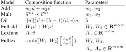
Table 1: Composition functions of inputs(u, v).
neighbor words or phrases) simultaneously. They use recursive neural networks to learn and con-struct the entire model and show that it reaches state-of-the-art performance in various evaluation experiments.
In this paper, we focus on the simpler, linear lexical function model proposed by Baroni and Zamparelli (2010) (see also Coecke et al. (2010)) and show that its performance can be further im-proved through more advanced regression tech-niques. We use the recently introduced elastic-net regularized linear regression method, which is solved by the pathwise coordinate descent opti-mization algorithm along a regularization parame-ter path. This new regression method can rapidly generate a sequence of solutions along the regular-ization path. Performing cross-validation on this parameter path should yield a much more accurate model for prediction. Besides better prediction ac-curacy, the elastic-net method also brings inter-pretability to the composition procedure through sparsity constraints on the model.
The rest of this paper is organized as follows: In Section 2, we give details on the above-mentioned composition models, which will be used for com-parison in our experiments. In Section 3, we de-scribe the pathwise optimized elastic-net regres-sion algorithm. Experimental evaluation on three composition tasks is provided in Section 4. In Sec-tion 5 we conclude and suggest direcSec-tions for fu-ture work.
2 Composition Models
Mitchell and Lapata (2008; 2010) present a set of simple but effective models in which each compo-nent of the output vector is a function of the cor-responding components of the inputs. Given in-put vectors⃗uand⃗v, the weighted additive model (Add) returns their weighted sum: ⃗p = w1⃗u+
w2⃗v. In the dilation model (Dil), the output vector
is obtained by decomposing one of the input vec-tors, say⃗v, into a vector parallel to ⃗uand an
or-thogonal vector, and then dilating only the parallel vector by a factorλbefore re-combining (formula in Table 1). Mitchell and Lapata also propose a simple multiplicative model in which the output components are obtained by component-wise mul-tiplication of the corresponding input components. We use its naturalweightedextension (Mult), in-troduced by Dinu et al. (2013), that takesw1 and
w2powers of the components before multiplying,
such that each phrase component pi is given by:
pi =uw1i viw2.
Guevara (2010) and Zanzotto et al. (2010) ex-plore a full form of the additive model (Fulladd), where the two vectors entering a composition pro-cess are pre-multiplied by weight matrices before being added, so that each output component is a weighted sum of all input components: ⃗p =
W1⃗u+W2⃗v.
Baroni and Zamparelli (2010) and Coecke et al. (2010), taking inspiration from formal seman-tics, characterize composition asfunction applica-tion. For example, Baroni and Zamparelli model adjective-noun phrases by treating the adjective as a regression function from nouns onto (mod-ified) nouns. Given that linear functions can be expressed by matrices and their application by matrix-by-vector multiplication, a functor (such as the adjective) is represented by a matrix Au
to be composed with the argument vector⃗v(e.g., the noun) by multiplication, returning thelexical function (Lexfunc) representation of the phrase: ⃗p=Au⃗v.
The method proposed by Socher et al. (2012) can be seen as a combination and non-linear ex-tension of Fulladd and Lexfunc (that Dinu and col-leagues thus calledFulllex) in whichbothphrase elements act as functors (matrices)andarguments (vectors). Given input terms uandv represented by (⃗u, Au) and (⃗v, Av), respectively, their
com-position vector is obtained by applying first a lin-ear transformation and then the hyperbolic tangent function to the concatenation of the productsAu⃗v
and Av⃗u (see Table 1 for the equation). Socher
and colleagues also present a way to construct ma-trix representations for specific phrases, needed to scale this composition method to larger con-stituents. We ignore it here since we focus on the two-word case.
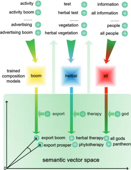
Figure 1: A sketch of the composition model train-ing and compostrain-ing procedure.
the case of the Fulladd and Lexfunc models this amounts to solving a multiple response multivari-ate regression problem.
The whole composition model training and phrase composition procedure is described with a sketch in Figure 1. To illustrate with an example, given an intransitive verbboom, we want to train a model for this intransitive verb so that we can use it for composition with a noun subject (e.g., export) to form an intransitive sentence (e.g., ex-port boom(s)). We treat these steps as a composi-tion model learning and predicting procedure. The training dataset is formed with pairs of input (e.g., activity) and output (e.g., activity boom) vectors. All composition models except Lexfunc also use the functor vector (boom) in the training data. Lex-func does not use this Lex-functor vector, but it would rather like to encode the learning target’s vector meaning in a different way (see experimental anal-ysis in Section 4.3). Then, this dataset is used for parameter estimation of models. When a model (boom) is trained and given a new input seman-tic vector (e.g.,export), it will output another vec-tor representing the concept forexport boom. And the conceptexport boomshould be close to simi-lar concepts (e.g.,export prosper) in meaning
un-der some distance metric in semantic vector space. The same training and composition scheme is ap-plied for other types of functors (e.g., adjectives and determiners). All the above mentioned com-position models are evaluated within this scheme, but note that in the case of Add, Dil, Mult and Ful-ladd, a single set of parameters is obtained across all functors of a certain syntactic category.
3 Pathwise Optimized Elastic-net Algorithm
The elastic-net regression method (Zou and Hastie, 2005) is proposed as a compromise be-tween lasso (Tibshirani, 1996) and ridge regres-sion (Hastie et al., 2009). Suppose there are N observation pairs(xi, yi), herexi ∈Rp is theith
training sample andyi ∈ Ris the corresponding
response variable in the typical regression setting. For simplicity, assume the xij are standardized:
∑N
i=1x2ij = 1, forj = 1, . . . , p. The elastic-net
solves the following problem:
min
(β0,β)∈Rp+1
[ 1
N
N
∑
i=1
(yi−β0−xTi β)2+λPα(β)
]
(1) where
Pα(β) = λ((1−α)12 ∥β ∥2ℓ2 +αβℓ1)
=
p
∑
j=1
[1
2(1−α)βj2+α|βj|].
P is the elastic-net penalty, and it is a compro-mise between the ridge regression penalty and the lasso penalty. The merit of the elastic-net penalty depends on two facts: the first is that elastic-net in-herits lasso’s characteristic to shrink many of the regression coefficients to zero, a property called sparsity, which results in better interpretability of model; the second is that elastic-net inherits ridge regression’s property of a grouping effect, which means important correlated features can be con-tained in the model simultaneously, and not be omitted as in lasso.
method for the regularization parameter path, and they also provided a solution for elastic-net. The main idea of pathwise coordinate descent is to solve the penalized regression problem along an entire path of values for the regularization param-etersλ, using the current estimates as warm starts. The idea turns out to be quite efficient for elastic-net regression. The procedure can be described as below: firstly establish an 100 λ value sequence in log scale, and for each of the 100 regulariza-tion parameters, use the following coordinate-wise updating rule to cycle around the features for es-timating the corresponding regression coefficients until convergence.
˜
βj ←
S(1 N
∑N
i=1xij(yi−y˜(j)i ), λα
)
1 +λ(1−α) (2)
where
• y˜(j)i = ˜β0+∑ℓ̸=jxiℓβ˜ℓis the fitted value
ex-cluding the contribution fromxij, and hence
yi−y˜(j)i the partial residual for fittingβj.
• S(z, γ)is the soft-thresholding operator with value
S(z, γ) = sign(z)(|z| −γ)+
=
z−γ ifz >0andγ <|z|
z+γ ifz <0andγ <|z| 0 ifγ ≥ |z|
Then solutions for a decreasing sequence of val-ues forλare computed in this way, starting at the smallest value λmax for which the entire
coeffi-cient vector βˆ = 0. Then, 10-fold cross valida-tion on this regularizavalida-tion path is used to deter-mine the best model for prediction accuracy. The αparameter controls the model sparsity (the num-ber of coefficients equal to zero) and grouping ef-fect (shrinking highly correlated features simulta-neously).
In what follows, we call the elastic-net regres-sion lexical function model EnetLex. In Sec-tion 4, we will report the experiment results by EnetLex with α = 1. It equals to pathwise co-ordinate descent optimized lasso, which favours sparser solutions and is often a better estimator when the number of training samples is far greater than the number of feature dimensions, as in our case. We also experimented with intermediate α values (e.g.,α = 0.5), that were, consistently, in-ferior or equal to the lasso setting.
−2 0 2 4
200
400
600
800
log(Lambda)
Mean−Squared Error
[image:4.595.307.516.63.195.2]50 50 50 50 50 50 50 50 50 48 29 21 12 7 4 2 Model selection procedure for ’EnetLex’
Figure 2: Example of model selection procedure for elastic-net regression (“the” model for deter-miner phrase experiment, SVD, 50 dimensions).
Figure 2 is an example of the model selection procedure between different regularization param-eterλvalues for determiner “the” (experimental details are described in section 4). When α is fixed, EnetLex first generates a λsequence from λmax to λmin (λmax is set to the smallest value
which will shrink all the regression coefficients to zero, λmin = 0.0001) in log scale (rightmost
point in the plot). The red points corresponding to eachλvalue in the plot represent mean cross-validated errors and their standard errors. To esti-mate a model corresponding to someλvalue ex-cept λmax, we use the solution from previous λ
value as the initial coefficients (the warm starts mentioned before) for iteration with coordinate descent. This will often generate a stable solu-tion path for the wholeλsequence very fast. And we can choose the model with minimum cross-validation error on this path and use it for more accurate prediction. In Figure 2, the labels on the top are numbers of corresponding selected vari-ables (features), the right vertical dotted line is the largest value of lambda such that error is within 1 standard error of the minimum, and the left verti-cal dotted line corresponds to the λvalue which gives minimum cross-validated error. In this case, the λ value of minimum cross-validated error is 0.106, and its log is -2.244316. In all of our ex-periments, we will select models corresponding to minimum training-data cross-validated error.
4 Experiments
4.1 Datasets
direct point of comparison.
Intransitive sentences The first dataset, intro-duced by Mitchell and Lapata (2010), focuses on the composition of intransitive verbs and their noun subjects. It contains a total of 120 sentence pairs together with human similarity judgments on a 7-point scale. For example,value slumps/value declines is scored 7, skin glows/skin burns is scored 1. On average, each pair is rated by 30 participants. Rather than evaluating against mean scores, we use each rating as a separate data point, as done by Mitchell and Lapata. We report Spear-man correlations between huSpear-man-assigned scores and cosines of model-generated vector pairs.
Adjective-noun phrases Turney (2012) intro-duced a dataset including both noun-noun com-pounds and adjective-noun phrases (ANs). We fo-cus on the latter, and we frame the task as in Dinu et al. (2013). The dataset contains 620 ANs, each paired with a single-noun paraphrase. Examples include:upper side/upside,false belief/fallacyand electric refrigerator/fridge. We evaluate a model by computing the cosine of all 20K nouns in our semantic space with the target AN, and looking at the rank of the correct paraphrase in this list. The lower the rank, the better the model. We report median rank across the test items.
Determiner phrases The third dataset, intro-duced in Bernardi et al. (2013), focuses on a class of determiner words. It is a multiple-choice test where target nouns (e.g.,omniscience) must be matched with the most closely related determiner(-noun) phrases (DPs) (e.g., all knowl-edge). There are 173 target nouns in total, each paired with one correct DP response, as well as 5 foils, namely the determiner (all) and noun (knowledge) from the correct response and three more DPs, two of which contain the same noun as the correct phrase (much knowledge, some knowl-edge), the third the same determiner (all prelimi-naries). Other examples of targets/related-phrases are quatrain/four lines and apathy/no emotion. The models compute cosines between target noun and responses and are scored based on their accu-racy at ranking the correct phrase first.
4.2 Setup
We use a concatenation of ukWaC, Wikipedia (2009 dump) and BNC as source corpus,
total-Model Reduction Dim Correlation
Add NMF 150 0.1349
Dil NMF 300 0.1288
Mult NMF 250 0.2246
Fulladd SVD 300 0.0461
Lexfunc SVD 250 0.2673
Fulllex NMF 300 0.2682
EnetLex SVD 250 0.3239
Table 2: Best performance comparison for intran-sitive verb sentence composition.
ing 2.8 billion tokens.1 Word co-occurrences are
collected within sentence boundaries (with a max-imum of a 50-words window around the target word). Following Dinu et al. (2013), we use the top 10K most frequent content lemmas as context features, Pointwise Mutual Information as weight-ing method and we reduce the dimensionality of the data by both Non-negative Matrix Factoriza-tion (NMF, Lee and Seung (2000)) and Singular Value Decomposition (SVD). For both data di-mensionality reduction techniques, we experiment with different numbers of dimension varying from 50 to 300 with a step of 50. Since the Mult model works very poorly when the input vectors contain negative values, as is the case with SVD, for this model we report result distributions across the 6 NMF variations only.
We use the DIStributional SEmantics Compo-sition Toolkit (DISSECT)2which provides
imple-mentations for all models we use for comparison. Following Dinu and colleagues, we used ordinary least-squares to estimate Fulladd and ridge for Lexfunc. The EnetLex model is implemented in R with support from the glmnet package,3which
im-plements pathwise coordinate descent elastic-net regression.
4.3 Experimental Results and Analysis The experimental results are shown in Ta-bles 2, 3, 4 and Figures 3, 4, 5. The best per-formances from each model on the three compo-sition tasks are shown in the tables. The over-all result distributions across reduction techniques and dimensionalities are displayed in the figure
1http://wacky.sslmit.unibo.it;
http://www.natcorp.ox.ac.uk
2http://clic.cimec.unitn.it/composes/
toolkit/
3http://cran.r-project.org/web/
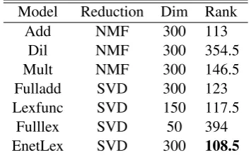
Model Reduction Dim Rank
Add NMF 300 113
Dil NMF 300 354.5
Mult NMF 300 146.5
Fulladd SVD 300 123 Lexfunc SVD 150 117.5
Fulllex SVD 50 394
[image:6.595.92.270.63.173.2]EnetLex SVD 300 108.5
Table 3: Best performance comparison for adjec-tive noun composition (lower ranks mean better performance).
Model Reduction Dim Rank
Add NMF 100 0.3237
Dil NMF 100 0.3584
Mult NMF 300 0.2023
[image:6.595.312.522.66.193.2]Fulladd NMF 200 0.3642 Lexfunc SVD 200 0.3699 Fulllex SVD 100 0.3699 EnetLex SVD 250 0.4046
Table 4: Best performance comparison for deter-miner phrase composition.
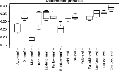
boxplots (NMF and SVD results are shown sep-arately). From Tables 2, 3, 4, we can see that EnetLex consistently achieves the best composi-tion performance overall, also outperforming the standard lexical function model. In the boxplot display, we can see that SVD is in general more stable across dimensionalities, yielding smaller variance in the results than NMF. We also observe, more specifically, larger variance in EnetLex per-formance on NMF than in Lexfunc, especially for determiner phrase composition. The large vari-ance with EnetLex comes from the NMF low-dimensionality results, especially the 50 dimen-sions condition. The main reason for this lies in the fast-computing tricks of the coordinate de-scent algorithm when cycling around many fea-tures with zero values (as resulting from NMF), which cause fast convergence at the beginning of the regularization path, generating an inaccurate model. A subordinate reason might lie in the un-standardized larger values of the NMF features (causing large gaps between adjacent parameter values in the regularization path). Although data standardization or other feature scaling techniques are often adopted in statistical analysis, they are seldom used in semantic composition tasks due to
Add−nmf Dil−nmf Mult−nmf Fulladd−nmf Le
xfunc−nmf
Fullle
x−nmf
EnetLe
x−nmf
Add−svd Dil−svd Mult−svd Fulladd−svd Le
xfunc−svd Fullle
x−svd
EnetLe
x−svd
0.00 0.05 0.10 0.15 0.20 0.25 0.30
Intransitive sentences
Figure 3: Intransitive verb sentence composition results.
Add−nmf Dil−nmf Mult−nmf Fulladd−nmf Le
xfunc−nmf Fullle
x−nmf
EnetLe
x−nmf
Add−svd Dil−svd Mult−svd Fulladd−svd Le
xfunc−svd Fullle
x−svd
EnetLe
x−svd
800 600 400 200 0
Adjective−noun phrases
Figure 4: Adjective noun phrase composition re-sults.
the fact that they might negatively affect the se-mantic vector space. A reasonable way out of this problem would be to save the mean and standard deviation parameters used for data standardization and use them to project the composed phrase vec-tor outputs back to the original vecvec-tor space.
On the other hand, EnetLex obtained a stable good performance in SVD space, with the best re-sults achieved with dimensions between 200 and 300. A set of Tukey’s Honestly Significant Tests show that EnetLex significantly outperforms the other models across SVD settings for determiner phrases and intransitive sentences. The difference is not significant for most comparisons in the ad-jective phrases task.
[image:6.595.312.522.254.385.2]Add−nmf Dil−nmf Mult−nmf Fulladd−nmf Le
xfunc−nmf
Fullle
x−nmf
EnetLe
x−nmf
Add−svd Dil−svd Mult−svd Fulladd−svd Le
xfunc−svd Fullle
x−svd
EnetLe
x−svd
0.15 0.20 0.25 0.30 0.35 0.40
[image:7.595.76.287.67.194.2]Determiner phrases
Figure 5: Determiner phrase composition results.
model verb adjective determiner Add 0.0259 957 0.2832 Mult 0.1796 298.5 0.0405 Table 5: Performance of Add and Mult models without dimensionality reduction.
results confirm that dimensionality reduction is not only a computational necessity when work-ing with more complex models, but it is actually improving the quality of the underlying semantic space.
Another benefit that elastic-net has brought to us is the sparsity in coefficient matrices. Sparsity here means that many entries in the coefficient ma-trix are shrunk to 0. For the above three exper-iments, the mean adjective, verb and determiner models’ sparsity ratios are 0.66, 0.55 and 0.18 re-spectively. Sparsity can greatly reduce the space needed to store the lexical function model, espe-cially when we want to use higher orders of repre-sentation. Moreover, sparsity in the model is help-ful to interpret the concept a specific functor word is conveying. For example, we show how to an-alyze the coefficient matrices for functor content words (verbs and adjectives). The verbburst and adjective poisonous, when estimated in the space projected to 100 dimensions with NMF, have per-centages of sparsity 47% and 39% respectively, which means 47% of the entries in theburst ma-trix and 39% of the entries in thepoisonous ma-trix are zeros.4 Most of the (hopefully) irrelevant
dimensions were discarded during model training. For visualization, we list the 6 most significant
4We analyze NMF rather than the better-performing SVD
features because the presence of negative values in the latter makes their interpretation very difficult. And NMF achieves comparably good performance for interpretation when di-mension exceeds 100.
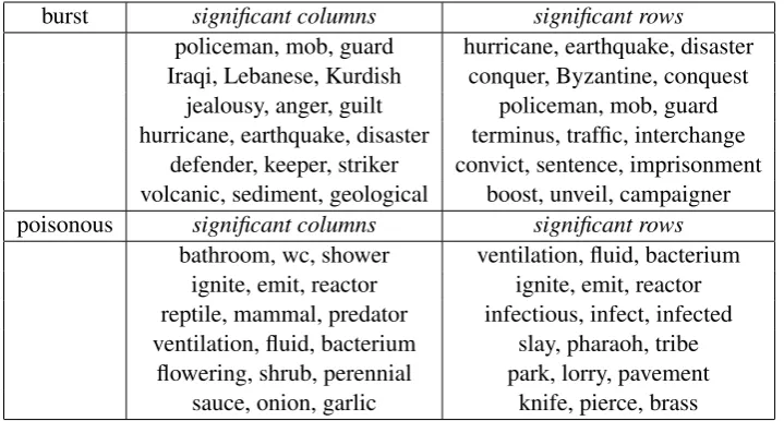
columns and rows from verb burst and adjective poisonous in Table 6. Each reduced NMF di-mension is represented by the 3 largest original-context entries in the corresponding row of the NMF basis matrix. The top columns and rows are selected by ordering sums of row entries and sums of column entries (the 10 most common fea-tures across trained matrices are omitted). In the matrix-vector multiplication scenario, a larger col-umn contributes more to all the features of the composed output phrase vector, while one large row corresponds to a large composition output fea-ture. From these tables, we can see that the se-lected top columns and rows are mostly semanti-cally relevant to the corresponding functor words (burstandpoisonous, in the displayed examples).
A very interesting aspect of these experiments is the role of the intercept in our regression model. The path-wise optimization algorithm starts with a lambda value (λmax), which sets all the
coef-ficients exactly to 0, and at that time the inter-cept is just the expected mean value of the train-ing phrase vectors, which in turn is of course quite similar to the co-occurrence vector of the cor-responding functor word (by averaging the poi-sonous N context distributions, we obtain a vec-tor that approximates thepoisonous distribution). And, although the intercept also changes with dif-ferent lambda values, it still highly correlates with the co-occurrence vectors of the functor words in vector space. For adjectives and verbs, we compared the initial model’s (λmax) intercept and
the minimum cross-validation error model inter-cept with corpus-extracted vectors for the corre-sponding words. That is, we used the word co-occurrence vector for a verb or an adjective ex-tracted from the corpus and projected onto the reduced feature space (e.g., NMF, 100 dimen-sions), then computed cosine similarity between this word meaning representation and its corre-sponding EnetLex matrix initial and minimum-error intercepts, respectively. Most of the simi-larities are still quite high after estimation: The mean cosine values for adjectives are 0.82 for the initial intercept and 0.72 for the minimum-error one. For verbs, the corresponding values are 0.75 and 0.69, respectively. Apparently, the sparsity constraint helps the intercept retaining information from training phrases.
burst significant columns significant rows policeman, mob, guard hurricane, earthquake, disaster Iraqi, Lebanese, Kurdish conquer, Byzantine, conquest
jealousy, anger, guilt policeman, mob, guard hurricane, earthquake, disaster terminus, traffic, interchange
defender, keeper, striker convict, sentence, imprisonment volcanic, sediment, geological boost, unveil, campaigner poisonous significant columns significant rows
bathroom, wc, shower ventilation, fluid, bacterium ignite, emit, reactor ignite, emit, reactor reptile, mammal, predator infectious, infect, infected ventilation, fluid, bacterium slay, pharaoh, tribe
[image:8.595.120.480.62.255.2]flowering, shrub, perennial park, lorry, pavement sauce, onion, garlic knife, pierce, brass
Table 6: Interpretability for verbs and adjectives (exemplified byburstandpoisonous).
vector space. For example, if we check the inter-cept forpoisonous, the cosine between the origi-nal vector space representation (from corpus) and the minimum-error solution intercept (from train-ing phrases) is at 0.7. The NMF dimensions cor-responding with the largest intercept entries are rather intuitive forpoisonous: ⟨ventilation, fluid, bacterium⟩, ⟨racist, racism, outrage⟩, ⟨reptile, mammal, predator⟩,⟨flowering, shrub, perennial⟩,
⟨sceptical, accusation, credibility⟩,⟨infectious, in-fect, infected⟩.
The mathematical reason for the above facts lies in the updating rule of the elastic-net’s intercept:
β0 = ¯y− p
∑
j=1
ˆ
βjx¯j (3)
Sparsity in the regression coefficients (βˆj)
encour-ages intercept β0 to stay as close to the mean
value of response y¯ as possible. So the elastic-net lexical function composition model isde facto also capturing the inherent meaning of the func-tor word, learning it from the training word-phrase pairs. In future research, we would like to test if these lexical meaning representations are as good or even better than standard co-occurrence vectors for single-word similarity tasks.
5 Conclusion
In this paper, we have shown that the lexical func-tion composifunc-tion model can be improved by ad-vanced regression techniques. We use pathwise coordinate descent optimized elastic-net, testing it on composing intransitive sentences,
adjective-noun phrases and determiner phrases in compari-son with other composition models, including lex-ical function estimated with ridge regression. The elastic-net method leads to performance gains on all three tasks. Through sparsity constraints on the model, elastic-net also introduces interpretability in the lexical function composition model. The regression coefficient matrices can often be eas-ily interpreted by looking at large row and column sums, as many matrix entries are shrunk to zero. The intercept of elastic-net regression also plays an interesting role in the model. With the sparsity constraints, the intercept of the model tends to re-tain the inherent meaning of the word by averaging training phrase vectors.
Our approach naturally generalizes to similar composition tasks, in particular those involving higher-order tensors (Grefenstette et al., 2013), where sparseness might be crucial in producing compact representations of very large objects. Our results also suggest that the performance of the lexical function composition model might be fur-ther improved with even more advanced methods, such as nonlinear regression. In the future, we would also like to explore interpretability more in depth, by looking at grouping and interaction ef-fects between features.
Acknowledgments
References
Marco Baroni and Roberto Zamparelli. 2010. Nouns are vectors, adjectives are matrices: Representing adjective-noun constructions in semantic space. In
Proceedings of EMNLP, pages 1183–1193, Boston, MA.
Raffaella Bernardi, Georgiana Dinu, Marco Marelli, and Marco Baroni. 2013. A relatedness benchmark to test the role of determiners in compositional dis-tributional semantics. InProceedings of ACL (Short Papers), pages 53–57, Sofia, Bulgaria.
Stephen Clark. 2013. Vector space models of lexical meaning. In Shalom Lappin and Chris Fox, editors,
Handbook of Contemporary Semantics, 2nd edition. Blackwell, Malden, MA. In press.
Bob Coecke, Mehrnoosh Sadrzadeh, and Stephen Clark. 2010. Mathematical foundations for a com-positional distributional model of meaning. Linguis-tic Analysis, 36:345–384.
Georgiana Dinu, Nghia The Pham, and Marco Baroni. 2013. General estimation and evaluation of com-positional distributional semantic models. In Pro-ceedings of ACL Workshop on Continuous Vector Space Models and their Compositionality, pages 50– 58, Sofia, Bulgaria.
Bradley Efron, Trevor Hastie, Iain Johnstone, and Robert Tibshirani. 2004. Least angle regression.
The Annals of statistics, 32(2):407–499.
Katrin Erk. 2012. Vector space models of word mean-ing and phrase meanmean-ing: A survey. Language and Linguistics Compass, 6(10):635–653.
Peter Foltz, Walter Kintsch, and Thomas Landauer. 1998. The measurement of textual coherence with Latent Semantic Analysis. Discourse Processes, 25:285–307.
Jerome Friedman, Trevor Hastie, Holger H¨ofling, and Robert Tibshirani. 2007. Pathwise coordinate optimization. The Annals of Applied Statistics, 1(2):302–332.
Jerome Friedman, Trevor Hastie, and Rob Tibshirani. 2010. Regularization paths for generalized linear models via coordinate descent. Journal of statisti-cal software, 33(1):1.
Edward Grefenstette, Georgiana Dinu, Yao-Zhong Zhang, Mehrnoosh Sadrzadeh, and Marco Baroni. 2013. Multi-step regression learning for composi-tional distribucomposi-tional semantics. In Proceedings of IWCS, pages 131–142, Potsdam, Germany.
Tom Griffiths, Mark Steyvers, and Josh Tenenbaum. 2007. Topics in semantic representation. Psycho-logical Review, 114:211–244.
Emiliano Guevara. 2010. A regression model of adjective-noun compositionality in distributional se-mantics. In Proceedings of GEMS, pages 33–37, Uppsala, Sweden.
Trevor Hastie, Robert Tibshirani, and Jerome Fried-man. 2009. The Elements of Statistical Learning, 2nd ed. Springer, New York.
Darrell Laham. 1997. Latent Semantic Analysis approaches to categorization. In Proceedings of CogSci, page 979.
Daniel Lee and Sebastian Seung. 2000. Algorithms for Non-negative Matrix Factorization. InProceedings of NIPS, pages 556–562.
Scott McDonald and Chris Brew. 2004. A distribu-tional model of semantic context effects in lexical processing. In Proceedings of ACL, pages 17–24, Barcelona, Spain.
Jeff Mitchell and Mirella Lapata. 2008. Vector-based models of semantic composition. InProceedings of ACL, pages 236–244, Columbus, OH.
Jeff Mitchell and Mirella Lapata. 2010. Composition in distributional models of semantics. Cognitive Sci-ence, 34(8):1388–1429.
Richard Socher, Brody Huval, Christopher Manning, and Andrew Ng. 2012. Semantic compositionality through recursive matrix-vector spaces. In Proceed-ings of EMNLP, pages 1201–1211, Jeju Island, Ko-rea.
Rob Tibshirani. 1996. Regression shrinkage and se-lection via the lasso. Journal of the Royal Statistical Society. Series B (Methodological), 58(1):267–288. Peter Turney and Patrick Pantel. 2010. From
fre-quency to meaning: Vector space models of se-mantics. Journal of Artificial Intelligence Research, 37:141–188.
Peter Turney. 2012. Domain and function: A dual-space model of semantic relations and compositions.
J. Artif. Intell. Res.(JAIR), 44:533–585.
Fabio Zanzotto, Ioannis Korkontzelos, Francesca Falucchi, and Suresh Manandhar. 2010. Estimat-ing linear models for compositional distributional semantics. InProceedings of COLING, pages 1263– 1271, Beijing, China.