Long Short Term Memory Neural Networks for Chinese Word Segmentation

Long Short-Term Memory Neural Networks

for Chinese Word Segmentation

Xinchi Chen, Xipeng Qiu∗, Chenxi Zhu, Pengfei Liu, Xuanjing Huang Shanghai Key Laboratory of Intelligent Information Processing, Fudan University

School of Computer Science, Fudan University 825 Zhangheng Road, Shanghai, China

{xinchichen13,xpqiu,czhu13,pfliu14,xjhuang}@fudan.edu.cn

Abstract

Currently most of state-of-the-art meth-ods for Chinese word segmentation are based on supervised learning, whose fea-tures are mostly extracted from a local con-text. These methods cannot utilize the long distance information which is also crucial for word segmentation. In this paper, we propose a novel neural network model for Chinese word segmentation, which adopts the long short-term memory (LSTM) neu-ral network to keep the previous impor-tant information in memory cell and avoids the limit of window size of local context. Experiments on PKU, MSRA and CTB6 benchmark datasets show that our model outperforms the previous neural network models and state-of-the-art methods.

1 Introduction

Word segmentation is a fundamental task for nese language processing. In recent years, Chi-nese word segmentation (CWS) has undergone great development. The popular method is to re-gard word segmentation task as a sequence label-ing problem (Xue, 2003; Peng et al., 2004). The goal of sequence labeling is to assign labels to all elements in a sequence, which can be handled with supervised learning algorithms such as Maximum Entropy (ME) (Berger et al., 1996) and Condi-tional Random Fields (CRF) (Lafferty et al., 2001). However, the ability of these models is restricted by the design of features, and the number of fea-tures could be so large that the result models are too large for practical use and prone to overfit on training corpus.

Recently, neural network models have increas-ingly used for NLP tasks for their ability to min-imize the effort in feature engineering (Collobert

∗_{Corresponding author.}

et al., 2011; Socher et al., 2013; Turian et al., 2010; Mikolov et al., 2013b; Bengio et al., 2003). Collobert et al. (2011) developed the SENNA sys-tem that approaches or surpasses the state-of-the-art systems on a variety of sequence labeling tasks for English. Zheng et al. (2013) applied the archi-tecture of Collobert et al. (2011) to Chinese word segmentation and POS tagging, also he proposed a perceptron style algorithm to speed up the train-ing process with negligible loss in performance. Pei et al. (2014) models tag interactions, tag-character interactions and tag-character-tag-character in-teractions based on Zheng et al. (2013). Chen et al. (2015) proposed a gated recursive neural network (GRNN) to explicitly model the combinations of the characters for Chinese word segmentation task. Each neuron in GRNN can be regarded as a differ-ent combination of the input characters. Thus, the whole GRNN has an ability to simulate the design of the sophisticated features in traditional methods. Despite of their success, a limitation of them is that their performances are easily affected by the size of the context window. Intuitively, many words are difficult to segment based on the local information only. For example, the segmentation of the following sentence needs the information of the long distance collocation.

冬 天 (winter)， 能 (can) 穿 (wear) 多 少 (amount) 穿 (wear) 多 少 (amount)； 夏 天 (summer)，能(can)穿(wear)多(more)少 (little)穿(wear)多(more)少(little)。

Without the word “夏天 (summer)” or “冬天 (winter)”, it is difficult to segment the phrase “能

穿多少穿多少”. Therefore, we usually need uti-lize the non-local information for more accurate word segmentation. However, it does not work by simply increasing the context window size. As reported in (Zheng et al., 2013), the performance drops smoothly when the window size is larger than 3. The reason is that the number of its pa-rameters is so large that the trained network has

overfitted on training data. Therefore, it is neces-sary to capture the potential long-distance depen-dencies without increasing the size of the context window.

In order to address this problem, we propose a neural model based on Long Short-Term Memory Neural Network (LSTM) (Hochreiter and Schmid-huber, 1997) that explicitly model the previous information by exploiting input, output and for-get gates to decide how to utilize and update the memory of pervious information. Intuitively, if the LSTM unit detects an important feature from an input sequence at early stage, it easily carries this information (the existence of the feature) over a long distance, hence, capturing the potential use-ful long-distance information. We evaluate our model on three popular benchmark datasets (PKU, MSRA and CTB6), and the experimental results show that our model achieves the state-of-the-art performance with the smaller context window size (0,2).

The contributions of this paper can be summa-rized as follows.

• We first introduce the LSTM neural network for Chinese word segmentation. The LSTM can capture potential long-distance depen-dencies and keep the previous useful informa-tion in memory, which avoids the limit of the size of context window.

• Although there are relatively few researches of applying dropout method to the LSTM, we investigate several dropout strategies and find that dropout is also effective to avoid the overfitting of the LSTM.

• Despite Chinese word segmentation being a specific case, our model can be easily gener-alized and applied to the other sequence la-beling tasks.

2 Neural Model for Chinese Word Segmentation

Chinese word segmentation is usually regarded as character-based sequence labeling. Each character is labeled as one of {B, M, E, S} to indicate the segmentation. {B, M, E} represent Begin, Mid-dle,Endof a multi-character segmentation respec-tively, and S represents aSinglecharacter segmen-tation.

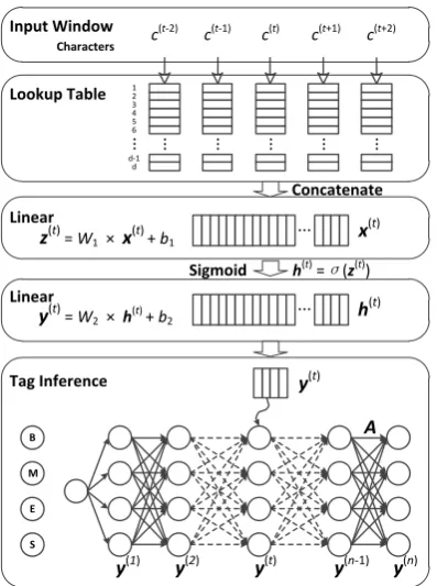
The neural model is usually characterized by three specialized layers: (1) a character embedding

layer; (2) a series of classical neural network lay-ers and (3) tag inference layer. An illustration is shown in Figure 1.

The most common tagging approach is based on a local window. The window approach as-sumes that the tag of a character largely depends on its neighboring characters. Given an input sen-tence c(1:n), a window of size k slides over the sentence from character c(1) to c(n), where n is the length of the sentence. As shown in Figure 1, for each character c(t)(1 ≤ t ≤ n), the con-text characters (c(t−2),c(t−1),c(t),c(t+1),c(t+2)) are fed into the lookup table layer when the window size k is 5. The characters exceeding the sen-tence boundaries are mapped to one of two spe-cial symbols, namely “start” and “end” symbols. The character embeddings extracted by the lookup table layer are then concatenated into a single vec-tor x(t) ∈ RH1_{, where} H₁ = k ×d_{is the size}

of layer 1. Then x(t) is fed into the next layer which performs linear transformation followed by an element-wise activation functiongsuch as sig-moid functionσ(x) = (1+e−x)−1and hyperbolic tangent functionϕ(x) = e_ex_x−_+ee₋−x_xhere.

h(t)=g(W₁x(t)+b₁), (1)

whereW₁∈RH2×H1_,b1∈RH2_,h(t) _∈RH2_{. H2}

is a hyper-parameter which indicates the number of hidden units in layer 2. Given a set of tagsT of size |T |, a similar linear transformation is performed except that no non-linear function is followed:

y(t) =W₂h(t)+b₂, (2)

whereW₂ ∈ R|T |×H2_,b2 ∈ R|T |_{. y}(t) ∈ R|T |_is

the score vector for each possible tag. In Chinese word segmentation, the most prevalent tag setT j T is {B, M, E, S} as mentioned above.

To model the tag dependency, a transition score

A_ij is introduced to measure the probability of jumping from tagi ∈ T to tagj ∈ T (Collobert et al., 2011). Although this model works well for Chinese word segmentation and other sequence la-beling tasks, it just utilizes the information of con-text of a limited-length window. Some useful long distance information is neglected.

3 Long Short-Term Memory Neural Network for Chinese Word

Segmentation

…

d-1 d 3 4 5 2

6 1

…

… Characters

Input Window

Lookup Table

Linear

x(t)

Sigmoid

z(t) = W1 × x(t)+ b1

h(t)

Linear

y(t) = W2 × h(t)+ b2

h(t) =σ(z(t))

Concatenate

Tag Inference

B

M

E

S

y(t) y(2)

y(1) y(n-1) y(n)

A y(t)

c(t-2) _c(t-1) _c(t) _c(t+1) _c(t+2)

… … … … …

Figure 1: General architecture of neural model for Chinese word segmentation.

3.1 Character Embeddings

The first step of using neural network to process symbolic data is to represent them into distributed vectors, also called embeddings (Bengio et al., 2003; Collobert and Weston, 2008).

Formally, in Chinese word segmentation task, we have a character dictionaryC of size |C|. Un-less otherwise specified, the character dictionary is extracted from the training set and unknown char-acters are mapped to a special symbol that is not used elsewhere. Each character c ∈ C is repre-sented as a real-valued vector (character embed-ding)v_c∈Rdwheredis the dimensionality of the vector space. The character embeddings are then stacked into an embedding matrixM∈Rd×|C|. For a characterc∈ C, the corresponding character em-beddingv_c ∈ Rdis retrieved by the lookup table layer. And the lookup table layer can be regarded as a simple projection layer where the character embedding for each context character is achieved by table lookup operation according to its index.

3.2 LSTM

The long short term memory neural network (LSTM) (Hochreiter and Schmidhuber, 1997) is an extension of the recurrent neural network (RNN).

The RNN has recurrent hidden states whose output at each time is dependent on that of the previous time. More formally, given a sequence

x(1:n) = (x(1),x(2), . . . ,x(t), . . . ,x(n)), the RNN updates its recurrent hidden stateh(t)by

h(t)=g(Uh(t−1)+Wx(t)+b), (3)

where g is a nonlinear function as mentioned above.

Though RNN has been proven successful on many tasks such as speech recognition (Vinyals et al., 2012), language modeling (Mikolov et al., 2010) and text generation (Sutskever et al., 2011), it can be difficult to train them to learn long-term dynamics, likely due in part to the vanishing and exploding gradient problem (Hochreiter and Schmidhuber, 1997).

The LSTM provides a solution by incorporating memory units that allow the network to learn when to forget previous information and when to update the memory cells given new information. Thus, it is a natural choice to apply LSTM neural network to word segmentation task since the LSTM neural network can learn from data with long range tem-poral dependencies (memory) due to the consider-able time lag between the inputs and their corre-sponding outputs. In addition, the LSTM has been applied successfully in many NLP tasks, such as text classification (Liu et al., 2015) and machine translation (Sutskever et al., 2014).

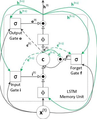
The core of the LSTM model is a memory cell

cencoding memory at every time step of what in-puts have been observed up to this step (see Figure 2) . The behavior of the cell is controlled by three “gates”, namely input gatei, forget gatefand out-put gateo. The operations on gates are defined as element-wise multiplications, thus gate can either scale the input value if the gate is non-zero vector or omit input if the gate is zero vector. The output of output gate will be fed into the next time step

t+ 1as previous hidden state and input of upper layer of neural network at current time stept. The definitions of the gates, cell update and output are as follows:

i(t)=σ(Wixx(t)+W_ihh(t−1)+Wicc(t−1)), (4)

f(t)=σ(Wfxx(t)+Wfhh(t−1)+Wfcc(t−1)), (5)

c(t)=f(t)⊙c(t−1)+i(t)⊙ϕ(Wcxx(t)+Wchh(t−1)), (6)

o(t)=σ(Woxx(t)+Wohh(t−1)+Wocc(t)), (7)

x(t) c

σ

σ

σ

φ

φ

Output Gate o

Input Gate i

Forget Gate f

LSTM Memory Unit c(t-1)

c(t-1)

c(t)

c(t) c(t-1)

o(t)

i(t)

f(t) h(t) h(t-1)

h(t-1) h(t-1)

h(t-1)

Figure 2: LSTM Memory Unit. The memory unit contains a cellcwhich is controlled by three gates. The green links show the signals at time t −1, while the black links show the current signals. The dashed links represent the weight matrices from beginning to end are diagonal. Moreover, the solid pointers mean there are weight matrices on the connections, and hollow pointers mean none. The current output signal,h(t), will fed back to the next timet+ 1 via three gates, and is the input of the higher layer of the neural network as well.

whereσandϕare the logistic sigmoid function and hyperbolic tangent function respectively;i(t),f(t),

o(t)andc(t)are respectively the input gate, forget gate, output gate, and memory cell activation vec-tor at time stept, all of which have the same size as the hidden vectorh(t) ∈ RH2_{; the parameter}

ma-trices Ws with different subscripts are all square matrices; ⊙denotes the element-wise product of the vectors. Note thatW_ic,W_fc andW_ocare di-agonal matrices.

3.3 LSTM Architectures for Chinese Word

Segmentation

To fully utilize the LSTM, we propose four differ-ent structures of neural network to select the effec-tive features via memory units. Figure 3 illustrates our proposed architectures.

LSTM-1 The LSTM-1 simply replace the

hid-den neurons in Eq. (1) with LSTM units (See Fig-ure 3a).

The input of the LSTM unit is from a window of context characters. For each character, c(t),(1 ≤

t≤n), the input of the LSTM unitx(t),

x(t)=v_c(t−k1)⊕ · · · ⊕v_c(t+k2), (9)

is concatenated from character embeddings of

c(t−k1):(t+k2)_{, wherek1andk2represent the}

num-bers of characters from left and right contexts re-spectively. The output of the LSTM unit is used in final inference function (Eq. (11) ) after a linear transformation.

LSTM-2 The LSTM-2 can be created by

stack-ing multiple LSTM hidden layers on top of each other, with the output sequence of one layer form-ing the input sequence for the next (See Figure 3b). Here we use two LSTM layers. Specifically, input of the upper LSTM layer takesh(t)from the lower LSTM layer without any transformation. The in-put of the first layer is same to LSTM-1, and the output of the second layer is as same operation as LSTM-1.

LSTM-3 The 3 is a extension of

LSTM-1, which adopts a local context of LSTM layer as input of the last layer (See Figure 3c). For each time stept, we concatenate the outputs of a win-dow of the LSTM layer into a vectorhˆ(t),

ˆ

h(t)=h(t−m1)⊕ · · · ⊕h(t+m2), (10)

wherem₁andm₂represent the lengths of time lags

before and after current time step.Finally, hˆ(t) is used in final inference function (Eq. (11) ) after a linear transformation.

LSTM-4 The LSTM-4 (see Figure 3d) is a mix-ture of the LSTM-2 and LSTM-3, which consists of two LSTM layers. The output sequence of the lower LSTM layer forms the input sequence of the upper LSTM layer. The final layer adopts a local context of upper LSTM layer as input.

3.4 Inference at Sentence Level

LSTM LSTM LSTM y(t-1)

y(t)

y(t+1)

x(t-1)

x(t)

x(t+1)

(a) LSTM-1

LSTM LSTM LSTM y(t-1)

y(t)

y(t+1)

x(t-1) _x(t) _x(t+1)

LSTM LSTM LSTM

(b) LSTM-2

LSTM LSTM LSTM y(t-1)

y(t)

y(t+1)

x(t-1)

x(t)

x(t+1)

(c) LSTM-3

LSTM LSTM LSTM y(t-1)

y(t)

y(t+1)

x(t-1)

x(t)

x(t+1)

LSTM LSTM LSTM

(d) LSTM-4

Figure 3: Our proposed LSTM architectures for Chinese word segmentation.

s(c(1:n)_{, y}(1:n)_{, θ) =}∑n

t=1

(

A_y(t−1)_y(t)+y(_yt()t) )

, (11)

where y(_yt₍)_t) indicates the score of tag y(t),

and y(t) is computed by the network as in Eq. (2). The parameter set of our model θ = {M,A,W_ic,W_fc,W_oc,W_ix,W_fx,W_ox,W_ih,W_fh, W_oh,W_cx,W_ch}.

4 Training

4.1 Max-Margin criterion

We use the Max-Margin criterion to train our model. Intuitively, the Max-Margin criterion pro-vides an alternative to probabilistic, likelihood based estimation methods by concentrating di-rectly on the robustness of the decision boundary of a model (Taskar et al., 2005). We useY(x_i)to denote the set of all possible tag sequences for a given sentencex_iand the correct tag sequence for

xi isyi. The parameter set of our model isθ. We

first define a structured margin loss ∆(y_i,yˆ) for predicted tag sequenceyˆ:

∆(yi,yˆ) = n

∑

t

η1{y_i(t)̸= ˆy(t)}, (12)

wherenis the length of sentencex_iandηis a dis-count parameter. The loss is proportional to the number of characters with incorrect tags in the pro-posed tag sequence. For a given training instance (x_i,y_i),the predicted tag sequenceyˆ_i ∈ Y(x_i)is the one with the highest score:

ˆ

yi=arg max

y∈Y(xi)

s(xi, y, θ), (13)

where the functions(·)is sentence-level score and defined in equation (11).

Given a set of training setD, the regularized ob-jective function is the loss functionJ(θ)including

al₂-norm term:

J(θ) = 1

|D| ∑

(xi,yi)∈D

li(θ) +λ₂∥θ∥22, (14)

where l_i(θ) = max(0, s(x_i,yˆ_i, θ) + ∆(y_i,yˆ_i) −

s(xi, yi, θ)).

To minimize J(θ), we use a generalization of gradient descent called subgradient method (Ratliff et al., 2007) which computes a gradient-like direction.

Following (Socher et al., 2013), we also use the diagonal variant of AdaGrad (Duchi et al., 2011) with minibatchs to minimize the objective. The parameter update for thei-th parameterθ_t,iat time steptis as follows:

θt,i =θt−1,i−√∑_tα τ=1gτ,i2

gt,i, (15)

whereαis the initial learning rate andg_τ ∈ R|θi| is the subgradient at time stepτ for parameterθ_i. In addition, the process of back propagation is fol-lowd Hochreiter and Schmidhuber (1997).

4.2 Dropout

Dropout is one of prevalent methods to avoid over-fitting in neural networks (Srivastava et al., 2014). When dropping a unit out, we temporarily remove it from the network, along with all its incoming and outgoing connections. In the simplest case, each unit is omitted with a fixed probabilityp indepen-dent of other units, namely dropout rate, wherep is also chosen on development set.

5 Experiments

5.1 Datasets

0 10 20 30 88

90 92 94 96

epoches

F-value(%)

Dropout Rate=20%

Dropout Rate=50%

without Dropout

(a) LSTM-1(2,2)

0 10 20 30

88 90 92 94 96

epoches

F-value(%)

Dropout Rate=20%

Dropout Rate=50%

without Dropout

(b) LSTM-1 (1,2)

0 10 20 30

88 90 92 94 96

epoches

F-value(%)

Dropout Rate=20%

Dropout Rate=50%

without Dropout

(c) LSTM-1(0,2)

Figure 4: Performances of LSTM-1 with the different context lengths and dropout rates on PKU devel-opment set.

Context length (k1, k2) = (0,2) Character embedding size d= 100

Hidden unit number H₂ = 150 Initial learning rate α= 0.2 Margin loss discount η = 0.2 Regularization λ= 10−4 Dropout rate on input layer p= 0.2

Table 1: Settings of the hyper-parameters.

0 20 40 60

80 85 90 95

epoches

F-value(%)

LSTM-1 LSTM-2

LSTM-3 LSTM-4

Figure 5: Performances of LSTM-1 (0,2) with 20% dropout on PKU development set.

and MSRA data are provided by the second In-ternational Chinese Word Segmentation Bakeoff (Emerson, 2005), and CTB6 is from Chinese Tree-Bank 6.0 (LDC2007T36) (Xue et al., 2005), which is a segmented, part-of-speech tagged and fully bracketed corpus in the constituency formalism. These datasets are commonly used by previous state-of-the-art models and neural network mod-els. In addition, we use the first 90% sentences of the training data as training set and the rest 10%

sentences as development set for PKU and MSRA datasets. For CTB6 dataset, we divide the training, development and test sets according to (Yang and Xue, 2012)

All datasets are preprocessed by replacing the Chinese idioms and the continuous English char-acters and digits with a unique flag.

For evaluation, we use the standard bake-off scoring program to calculate precision, recall, F1-score and out-of-vocabulary (OOV) word recall.

5.2 Hyper-parameters

Hyparameters of neural model impact the per-formance of the algorithm significantly. Accord-ing to experiment results, we choose the hyper-parameters of our model as showing in Figure 1. The minibatch size is set to 20. Generally, the number of hidden units has a limited impact on the performance as long as it is large enough. We found that 150 is a good trade-off between speed and model performance. The dimension-ality of character embedding is set to 100 which achieved the best performance. All these hyper-parameters are chosen according to their average performances on three development sets.

For the context lengths (k₁, k₂) and dropout strategy, we give detailed analysis in next section.

5.3 Dropout and Context Length

Context Length Dropout rate=20% Dropout rate=50% without Dropout

P R F P R F P R F

LSTM-1 (2,2) 95.8 95.3 95.6 94.8 94.4 94.6 95.2 94.9 95.1 LSTM-1 (1,2) 95.7 95.3 95.5 94.8 94.4 94.6 95.4 94.9 95.2 LSTM-1 (0,2) 95.8 95.5 95.7 94.6 94.2 94.4 95.4 95.0 95.2

Table 2: Performances of LSTM-1 with the different context lengths and dropout rates on PKU test set.

models Contextr Length = (0,2)

P R F

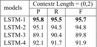
LSTM-1 95.8 95.5 95.7

LSTM-2 95.1 94.5 94.8 LSTM-3 89.1 90.4 89.8 LSTM-4 92.1 91.7 91.9

Table 3: Performance on our four proposed models on PKU test set.

Due to space constraints, we just give the per-formances of LSTM-1 model on PKU dataset with different context lengths(k₁, k₂)and dropout rates in Figure 4 and Table 2. From Figure 4, we can see that 20% dropout converges slightly slower than the one without dropout, but avoids overfitting. 50% or higher dropout rate seems to be underfit-ting since its training error is also high.

Table 2 shows that the LSTM-1 model performs consistently well with the different context length, but the LSTM-1 model with short context length saves computational resource, and gets more ef-ficiency. At the meanwhile, the LSTM-1 model with context length (0,2) can receive the same or better performance than that with context length (2,2), which shows that the LSTM model can well model the pervious information, and it is more ro-bust for its insensitivity of window size variation. We employ context length (0,2) with the 20% dropout rate in the following experiments to bal-ance the tradeoff between accuracy and efficiency.

5.4 Model Selection

We also evaluate the our four proposed models with the hyper-parameter settings in Table 1. For LSTM-3 and LSTM-4 models, the context win-dow length of top LSTM layer is set to (2,0). For LSTM-2 and LSTM-4,the number of upper hidden LSTM layer is set to 100. We use PKU dataset to select the best model. Figure 5 shows the results of the four models on PKU development set from first epoch to 60-th epoch. We see that the LSTM-1 is the fastest one to converge and achieves the best

performance. The LSTM-2 (two LSTM layers) get worse, which shows the performance seems not to benefit from deep model. The LSTM-3 and LSTM-4 models do not converge, which could be caused by the complexity of models.

The results on PKU test set are also shown in Ta-ble 3, which again show that the LSTM-1 achieves the best performance. Therefore, in the rest of the paper we will give more analysis based on the LSTM-1 with hyper-parameter settings as showing in Table 1.

5.5 Experiment Results

In this section, we give comparisons of the LSTM-1 with pervious neural models and state-of-the-art methods on the PKU, MSRA and CTB6 datasets.

We first compare our model with two neural models (Zheng et al., 2013; Pei et al., 2014) on Chinese word segmentation task with random ini-tialized character embeddings. As showing in Ta-ble 4, the performance is boosted significantly by utilizing LSTM unit. And more notably, our win-dow size of the context characters is set to (0,2), while the size of the other models is (2,2).

Previous works found that the performance can be improved by pre-training the character embed-dings on large unlabeled data. We use word2vec

1 _{(Mikolov et al., 2013a) toolkit to pre-train the}

character embeddings on the Chinese Wikipedia corpus. The obtained embeddings are used to ini-tialize the character lookup table instead of random initialization. Inspired by (Pei et al., 2014), we also utilize bigram character embeddings which is sim-ply initialized as the average of embeddings of two consecutive characters.

Table 5 shows the performances with addi-tional pre-trained and bigram character embed-dings. Again, the performances boost significantly as a result. Moreover, when we use bigram embed-dings only, which means we do close test without pre-training the embeddings on other extra corpus, our model still perform competitively compared

models PKU MSRA CTB6

P R F P R F P R F

(Zheng et al., 2013) 92.8 92.0 92.4 92.9 93.6 93.3 94.0* 93.1* 93.6* (Pei et al., 2014) 93.7 93.4 93.5 94.6 94.2 94.4 94.4* 93.4* 93.9*

LSTM 95.8 95.5 95.7 96.7 96.2 96.4 95.0 94.8 94.9

Table 4: Performances on three test sets with random initialized character embeddings. The results with * symbol are from our implementations of their methods.

models PKU MSRA CTB6

P R F P R F P R F

+Pre-train

(Zheng et al., 2013) 93.5 92.2 92.8 94.2 93.7 93.9 93.9* 93.4* 93.7* (Pei et al., 2014) 94.4 93.6 94.0 95.2 94.6 94.9 94.2* 93.7* 94.0* LSTM 96.3 95.6 96.0 96.7 96.5 96.6 95.9 95.5 95.7

+bigram

LSTM 96.3 95.9 96.1 97.1 97.1 97.1 95.6 95.3 95.5

+Pre-train+bigram

(Pei et al., 2014) - - 95.2 - - 97.2 - -

-LSTM 96.6 96.4 96.5 97.5 97.3 97.4 96.2 95.8 96.0

Table 5: Performances on three test sets with pre-trained and bigram character embeddings. The results with * symbol are from our implementations of their methods.

Models PKU MSRA CTB6

(Tseng et al., 2005) 95.0 96.4 -(Zhang and Clark, 2007) 95.1 97.2 -(Sun and Xu, 2011) - - 95.7 (Zhang et al., 2013) 96.1 97.4

-This work 96.5 97.4 96.0

Table 6: Comparison of our model with state-of-the-art methods on three test sets.

with previous neural models with pre-trained em-bedding and bigram emem-beddings.

Table 6 lists the performances of our model as well as previous state-of-the-art systems. (Zhang and Clark, 2007) is a word-based segmentation algorithm, which exploit features of complete words, while the rest of the list are character-based word segmenters, whose features are mostly ex-tracted from a window of characters. Moreover, some systems (such as Sun and Xu (2011) and Zhang et al. (2013)) also exploit kinds of extra in-formation such as unlabeled data or other knowl-edge. Despite our model only uses simple bigram features, it outperforms previous state-of-the-art models which use more complex features.

Since that we do not focus on the speed of the al-gorithm in this paper, we do not optimize the speed

a lot. On PKU dataset, it takes about 3 days to train the model (last row of Table 5) using CPU (Intel(R) Xeon(R) CPU E5-2665 @ 2.40GHz) only. All im-plementation is based on Python.

6 Related Work

Chinese word segmentation has been studied with considerable efforts in the NLP community. The most popular word segmentation methods is based on sequence labeling (Xue, 2003). Recently, re-searchers have tended to explore neural network based approaches (Collobert et al., 2011) to re-duce efforts of feature engineering (Zheng et al., 2013; Pei et al., 2014; Qi et al., 2014; Chen et al., 2015). The features of all these methods are ex-tracted from a local context and neglect the long distance information. However, previous informa-tion is also crucial for word segmentainforma-tion. Our model adopts the LSTM to keep the previous im-portant information in memory and avoids the lim-itation of ambiguity caused by limit of the size of context window.

7 Conclusion

long-distance features. Though our model use smaller context window size (0,2), it still outperforms the previous neural models with context window size (2,2). Besides, our model can also be easily gener-alized and applied to other sequence labeling tasks. Although our model achieves state-of-the-art performance, it only makes use of previous con-text. The future context is also useful for Chi-nese word segmentation. In future work, we would like to adopt the bidirectional recurrent neural net-work (Schuster and Paliwal, 1997) to process the sequence in both directions.

Acknowledgments

We would like to thank the anonymous review-ers for their valuable comments. This work was partially funded by the National Natural Science Foundation of China (61472088, 61473092), Na-tional High Technology Research and Develop-ment Program of China (2015AA015408), Shang-hai Science and Technology Development Funds (14ZR1403200).

References

Yoshua Bengio, Réjean Ducharme, Pascal Vincent, and Christian Janvin. 2003. A neural probabilistic lan-guage model. The Journal of Machine Learning Re-search, 3:1137–1155.

A.L. Berger, V.J. Della Pietra, and S.A. Della Pietra. 1996. A maximum entropy approach to natural language processing. Computational Linguistics, 22(1):39–71.

Xinchi Chen, Xipeng Qiu, Chenxi Zhu, and Xuanjing Huang. 2015. Gated recursive neural network for Chinese word segmentation. InProceedings of An-nual Meeting of the Association for Computational Linguistics.

Ronan Collobert and Jason Weston. 2008. A unified architecture for natural language processing: Deep neural networks with multitask learning. In Pro-ceedings of ICML.

Ronan Collobert, Jason Weston, Léon Bottou, Michael Karlen, Koray Kavukcuoglu, and Pavel Kuksa. 2011. Natural language processing (almost) from scratch. The Journal of Machine Learning Research, 12:2493–2537.

John Duchi, Elad Hazan, and Yoram Singer. 2011. Adaptive subgradient methods for online learning and stochastic optimization. The Journal of Machine Learning Research, 12:2121–2159.

T. Emerson. 2005. The second international Chi-nese word segmentation bakeoff. InProceedings of

the Fourth SIGHAN Workshop on Chinese Language Processing, pages 123–133. Jeju Island, Korea.

Sepp Hochreiter and Jürgen Schmidhuber. 1997. Long short-term memory. Neural computation, 9(8):1735–1780.

John D. Lafferty, Andrew McCallum, and Fernando C. N. Pereira. 2001. Conditional random fields: Probabilistic models for segmenting and labeling se-quence data. InProceedings of the Eighteenth Inter-national Conference on Machine Learning.

PengFei Liu, Xipeng Qiu, Xinchi Chen, Shiyu Wu, and Xuanjing Huang. 2015. Multi-timescale long short-term memory neural network for modelling sentences and documents. In Proceedings of the Conference on Empirical Methods in Natural Lan-guage Processing.

Tomas Mikolov, Martin Karafiát, Lukas Burget, Jan Cernockỳ, and Sanjeev Khudanpur. 2010. Recur-rent neural network based language model. In IN-TERSPEECH.

Tomas Mikolov, Kai Chen, Greg Corrado, and Jef-frey Dean. 2013a. Efficient estimation of word representations in vector space. arXiv preprint arXiv:1301.3781.

Tomas Mikolov, Ilya Sutskever, Kai Chen, Greg S Cor-rado, and Jeff Dean. 2013b. Distributed representa-tions of words and phrases and their compositional-ity. InNIPS, pages 3111–3119.

Wenzhe Pei, Tao Ge, and Chang Baobao. 2014. Max-margin tensor neural network for chinese word seg-mentation. InProceedings of ACL.

F. Peng, F. Feng, and A. McCallum. 2004. Chinese segmentation and new word detection using condi-tional random fields. Proceedings of the 20th inter-national conference on Computational Linguistics.

Yanjun Qi, Sujatha G Das, Ronan Collobert, and Jason Weston. 2014. Deep learning for character-based information extraction. InAdvances in Information Retrieval, pages 668–674. Springer.

Nathan D Ratliff, J Andrew Bagnell, and Martin A Zinkevich. 2007. (online) subgradient methods for structured prediction. InEleventh International Conference on Artificial Intelligence and Statistics (AIStats).

Mike Schuster and Kuldip K Paliwal. 1997. Bidirec-tional recurrent neural networks. Signal Processing, IEEE Transactions on, 45(11):2673–2681.

Nitish Srivastava, Geoffrey Hinton, Alex Krizhevsky, Ilya Sutskever, and Ruslan Salakhutdinov. 2014. Dropout: A simple way to prevent neural networks from overfitting. The Journal of Machine Learning Research, 15(1):1929–1958.

Weiwei Sun and Jia Xu. 2011. Enhancing Chinese word segmentation using unlabeled data. In Pro-ceedings of the Conference on Empirical Methods in Natural Language Processing, pages 970–979.

Ilya Sutskever, James Martens, and Geoffrey E Hin-ton. 2011. Generating text with recurrent neural networks. InProceedings of the 28th International Conference on Machine Learning (ICML-11), pages 1017–1024.

Ilya Sutskever, Oriol Vinyals, and Quoc VV Le. 2014. Sequence to sequence learning with neural networks. InAdvances in Neural Information Processing Sys-tems, pages 3104–3112.

Huihsin Tseng, Pichuan Chang, Galen Andrew, Daniel Jurafsky, and Christopher Manning. 2005. A condi-tional random field word segmenter for sighan bake-off 2005. In Proceedings of the fourth SIGHAN workshop on Chinese language Processing, volume 171.

Joseph Turian, Lev Ratinov, and Yoshua Bengio. 2010. Word representations: a simple and general method for semi-supervised learning. InProceedings of the 48th annual meeting of the association for compu-tational linguistics, pages 384–394. Association for Computational Linguistics.

Oriol Vinyals, Suman V Ravuri, and Daniel Povey. 2012. Revisiting recurrent neural networks for ro-bust asr. InAcoustics, Speech and Signal Processing (ICASSP), 2012 IEEE International Conference on, pages 4085–4088. IEEE.

Naiwen Xue, Fei Xia, Fu-Dong Chiou, and Martha Palmer. 2005. The Penn Chinese TreeBank: Phrase structure annotation of a large corpus. Natural lan-guage engineering, 11(2):207–238.

N. Xue. 2003. Chinese word segmentation as charac-ter tagging. Computational Linguistics and Chinese Language Processing, 8(1):29–48.

Yaqin Yang and Nianwen Xue. 2012. Chinese comma disambiguation for discourse analysis. In Proceed-ings of the 50th Annual Meeting of the Associa-tion for ComputaAssocia-tional Linguistics: Long Papers-Volume 1, pages 786–794. Association for Compu-tational Linguistics.

Yue Zhang and Stephen Clark. 2007. Chinese segmen-tation with a word-based perceptron algorithm. In

ACL.

Longkai Zhang, Houfeng Wang, Xu Sun, and Mairgup Mansur. 2013. Exploring representations from un-labeled data with co-training for Chinese word seg-mentation. InProceedings of the 2013 Conference

on Empirical Methods in Natural Language Process-ing.