Comparative Study Between Various Algorithms of Data Compression Techniques

Comparative Study Between

Various Algorithms of Data Compression Techniques

Mohammed Al-laham

_{& Ibrahiem M. M. El Emary}

1 Al Balqa Applied University, Amman, Jordan

2 Faculty of Engineering, Al Ahliyya Amman University, Amman, Jordan

E-mail: doctor_ebrahim@yahoo.com

Abstract

The spread of computing has led to an explosion in the volume of data to be stored on hard disks and sent over the Internet. This growth has led to a need for "data compression", that is, the ability to reduce the amount of storage or Internet bandwidth required to handle this data. This paper provides a survey of data compression techniques. The focus is on the most prominent data compression schemes, particularly popular .DOC, .TXT, .BMP, .TIF, .GIF, and .JPG files. By using different compression algorithms, we get some results and regarding to these results we suggest the efficient algorithm to be used with a certain type of file to be compressed taking into consideration both the compression ratio and compressed file size.

Keywords

RLE, RLL, HUFFMAN, LZ, LZW and HLZ

1. Introduction

The essential figure of merit for data compression is the "compression ratio", or ratio of the size of a compressed file to the original uncompressed file. For example, suppose a data file takes up 50 kilobytes (KB). Using data compression software, that file could be reduced in size to, say, 25 KB, making it easier to store on disk and faster to transmit over an Internet connection. In this specific case, the data compression software reduces the size of the data file by a factor of two, or results in a "compression ratio" of 2:1 [1, 2]. There are "lossless" and "lossy" forms of data compression. Lossless data compression is used when the data has to be uncompressed exactly as it was before compression. Text files are stored using lossless techniques, since losing a single character can be in the worst case make the text dangerously misleading. Archival storage of master sources for images, video data, and audio data generally needs to be lossless as well.

However, there are strict limits to the amount of compression that can be obtained with lossless compression. Lossless compression ratios are generally in the range of 2:1 to 8:1. [2, 3]. Lossy compression, in contrast, works on the assumption that the data doesn't have to be stored perfectly. Much information can be simply thrown away from images, video data, and audio data, and the when uncompressed; the data will still be of acceptable quality. Compression ratios can be an order of magnitude greater than those available from lossless methods.

The question of which are "better", lossless or lossy techniques is pointless. Each has its own uses, with lossless techniques better in some cases and lossy techniques better in others. In fact, as this paper will show, lossless and lossy techniques are often used together to obtain the highest compression ratios. Even given a specific type of file, the contents of the file, particularly the orderliness and redundancy of the data, can strongly influence the compression ratio. In some cases, using a particular data compression technique on a data file where there isn't a good match between the two can actually result in a bigger file [9].

2. Some Considerable Terminologies

A few little comments on terminology before we proceed are given as the following:

• Since most data compression techniques can work on different types of digital data such as characters or bytes in image files or whatever, data compression literature speaks in general terms of compressing "symbols".

a file. There's no strong distinction between the two as far as data compression is concerned. This paper also uses the term "message" in examples where short data strings are compressed [7, 10].

• Data compression literature also often refers to data compression as data "encoding", and of course that means data decompression is often

called "decoding". This paper tends to use the two sets of terms interchangeably.

3. Run Length Encoding Technique

One of the simplest forms of data compression is known as "run length encoding" (RLE), which is sometimes known as "run length limiting" (RLL) [8,10]. In this encoding technique, suppose you have a text file in which the same characters are often repeated one after another. This redundancy provides an opportunity for compressing the file. Compression software can scan through the file, find these redundant strings of characters, and then store them using an escape character (ASCII 27) followed by the character and a binary count of the number of times it is repeated. For example, the 50 character sequence:

XXXXXXXXXXXXXXXXXXXXXXXXXXXXXXX

that's all, folks!-- can be converted to: <ESC>X<31> . This eliminates 28 characters, compressing the text by more than a factor of two. Of course, the compression software must be smart enough not to compress strings of two or three repeated characters, since for three characters run length encoding would have no advantage, and for two it would actually increase the size of the output file.

As described, this scheme has two potential problems. First, an escape character may actually occur in the file. The answer is to use two escape characters to represent it, which can actually make the output file bigger if the uncompressed input file includes lots of escape characters. The second problem is that a single byte cannot specify run lengths greater than 256. This difficulty can be dealt by using multiple escape sequences to compress one very long string.

Run length encoding is actually not very useful for compressing text files since a typical text file doesn't have a lot of long, repetitive character

strings. It is very useful, however, for compressing bytes of a monochrome image file, which normally consists of solid black picture bits, or "pixels", in a sea of white pixels, or the reverse. Run-length encoding is also often used as a preprocessor for other compression algorithms.

4. HUFFMAN Coding Technique

A more sophisticated and efficient lossless compression technique is known as "Huffman coding", in which the characters in a data file are converted to a binary code, where the most common characters in the file have the shortest binary codes, and the least common have the longest [9]. To see how Huffman coding works, assume that a text file is to be compressed, and that the characters in the file have the following frequencies:

In practice, we need the frequencies for all the characters used in the text, including all letters, digits, and punctuation, but to keep the example simple we'll just stick to the characters from A to G.

The first step in building a Huffman code is to order the characters from highest to lowest frequency of occurrence as follows:

First, the two least-frequent characters are selected, logically grouped together, and their frequencies added. In this example, the D and E characters have a combined frequency of 21:

This begins the construction of a "binary tree" structure. We now again select the two elements the lowest frequencies, regarding the D-E combination as a single element. In this case, the two elements selected are G and the D-E combination. We group them together and add their frequencies. This new combination has a

44: We continue in the same way to select the two elements with the lowest frequency, group them together, and add their frequencies, until we run out of elements. In the third iteration, the lowest frequencies are C and A and the final binary tree will be as follows:

Tracing down the tree gives the "Huffman codes", with the shortest codes assigned

to the characters with the greatest frequency:

The Huffman codes won't get confused in decoding. The best way to see that this is so is to envision the decoder cycling through the tree structure, guided by the encoded bits it reads, moving from top to bottom and then back to the top. As long as bits constitute legitimate Huffman codes, and a bit doesn't get scrambled or lost, the decoder will never get lost, either. There is an alternate algorithm for generating these codes, known as Shannon-Fano coding. In fact, it preceded Huffman coding and one of the first data compression schemes to be devised, back in the 1950s. It was the work of the well-known Claude Shannon, working with R.M. Fano. David Huffman published a paper in 1952 that modified it slightly to create Huffman coding.]

5. ARITHMETIC Coding Technique

Huffman coding looks pretty slick, and it is, but there's a way to improve on it, known as "arithmetic coding". The idea is subtle and best explained by example [4, 8, 10]. Suppose we have a message that only contains the characters A, B, and C, with the following frequencies, expressed as fractions:

To show how arithmetic compression works, we first set up a table, listing characters with their probabilities along with the cumulative sum of those probabilities. The cumulative sum defines "intervals", ranging from the bottom value to less than, but not equal to, the top value. The order does not seem to be important.

Now each character can be coded by the shortest binary fraction that falls in the character's probability interval:

Sending one character is trivial and uninteresting. Let's consider sending messages consisting of all possible permutations of two of these three characters, using the same approach:

Obviously, this same procedure can be followed for more characters, resulting in a longer binary fractional value. What arithmetic coding does is find the

probability value of a particular message, and arrange it as part of a numerical order that allows its unique identification.

6. LZ-77 Encoding Technique [4, 5, 10]

Good as they are, Huffman and arithmetic coding are not perfect for encoding text because they don't capture the higher-order relationships between words and phrases. There is a simple, clever, and effective approach to compressing text known as LZ-77, which uses the redundant nature of text to provide compression. This technique was invented by two Israeli computer scientists, Abraham Lempel and Jacob Ziv, in 1977 [7,8,9,10].

LZ-77 exploits the fact that words and phrases within a text stream are likely to be repeated. When they do repeat, they can be encoded as a pointer to an earlier occurrence, with the pointer accompanied by the number of characters to be matched.

Pointers and uncompressed characters are distinguished by a leading flag bit, with a "0" indicating a pointer and a "1" indicating an uncompressed character. This means that uncompressed characters are extended from 8 to 9 bits, working against compression a little.

Key to the operation of LZ-77 is a sliding history buffer, also known as a "sliding window", which stores the text most recently transmitted. When the buffer fills up, its oldest contents are discarded. The size of the buffer is important. If it is too small, finding string matches will be less likely. If it is too large, the pointers will be larger, working against compression.

For an example, consider the phrase:

the_rain_in_Spain_falls_mainly_i n_the_plain

-- where the underscores ("_") indicate spaces. This uncompressed message is 43 bytes, or 344 bits, long.

At first, LZ-77 simply outputs uncompressed characters, since there are no previous occurrences of any strings to refer back to. In our example, these characters will not be compressed:

the_rain_

The next chunk of the message:

in_

-- has occurred earlier in the message, and can be represented as a pointer back to that earlier text, along with a length field. This gives:

the_rain_<3,3>

-- where the pointer syntax means "look back three characters and take three characters from that point." There are two different binary formats for the pointer:

• An 8 bit pointer plus 4 bit length, which assumes a maximum offset of 255 and a maximum length of 15.

• A 12 bit pointer plus 6 bit length, which assumes a maximum offset size of 4096, implying a 4 kilobyte buffer, and a maximum length of 63.

As noted, a flag bit with a value of 0 indicates a pointer. This is followed by a second flag bit giving the size of the pointer, with a 0 indicating an 8 bit pointer, and a 1 indicating a 12 bit pointer. So, in binary, the pointer <3,3> would look like this:

00 00000011 0011

The first two bits are the flag bits, indicating a pointer that is 8 bits long. The next 8 bits are the pointer value, while the last four bits are the length value.

After this comes:

-- which has to be output uncompressed:

the_rain_<3,3>Sp

However, the characters "ain_" have been sent, so they are encoded with a pointer:

the_rain_<3,3>Sp<9,4>

Notice here, at the risk of belaboring the obvious, that the pointers refer to offsets in the

uncompressed message. As the decoder receives

the compressed data, it uncompresses it, so it has access to the parts of the uncompressed message that the pointers reference.

The characters "falls_m" are output uncompressed, but "ain" has been used before in "rain" and "Spain", so once again it is encoded with a pointer:

the_rain_<3,3>Sp<9,4>fa lls_m<11,3>

Notice that this refers back to the "ain" in "Spain", and not the earlier "rain". This ensures

a smaller pointer.

The characters "ly" are output uncompressed, but "in_" and "the_" were output earlier, and so they are sent as pointers:

the_rain_<3,3>Sp<9,4>fa lls_m<11,3>ly_<16,3><34 ,4>

Finally, the characters "pl" are output

uncompressed, followed by another pointer to "ain". Our original message:

the_rain_in_Spain_falls _mainly_in_the_plain

-- has now been compressed into this form:

the_rain_<3,3>Sp<9,4>fa lls_m<11,3>ly_<16,3><34 ,4>pl<15,3>

This gives 23 uncompressed characters at 9 bits apiece, plus six 14 bit pointers, for a total of 291 bits as compared to the uncompressed text of 344 bits. This is not bad compression for such a short message, and of course compression gets better as the buffer fills up, allowing more matches.

LZ-77 will typically compress text to a third or less of its original size. The hardest part to implement is the search for matches in the buffer. Implementations use binary trees or hash tables to ensure a fast match. There are a several variations on the LZ-77, the best known being LZSS, which was published by Storer and Symanski in 1982. The differences between the two are unclear from the sources I have access to.

More drastic modifications of LZ-77 include a second level of compression on the output of the LZ-77 coder. LZH, for example, performs the second level of compression using Huffman coding, and is used in the popular LHA archiver. The ZIP algorithm, which is used in the popular PKZIP package and the freeware ZLIB compression library, uses Shannon-Fano coding for the second level of compression.

7. LZW Coding Technique

LZ-77 is an example of what is known as "substitutional coding". There are other schemes in this class of coding algorithms. Lempel and Ziv came up with an improved scheme in 1978, appropriately named LZ-78, and it was refined by a Mr. Terry Welch in 1984, making it LZW [6,8,10]. LZ-77 uses pointers to previous words or parts of words in a file to obtain compression. LZW takes that scheme one step further, actually constructing a "dictionary" of words or parts of words in a message, and then using pointers to the words in the dictionary. Let's go back to the example message used in the previous section:

the_rain_in_Spain_falls_ mainly_in_the_plain

The LZW algorithm stores strings in a "dictionary" with entries for 4,096 variable length strings. The first 255 entries are used to contain the values for individual bytes, so the actual first string index is 256. As the string is compressed, the dictionary is built up to contain every possible string combination that can be obtained from the message, starting with two characters, then three characters, and so on.

The next two-character string in the message is "in", but this has already been included in the dictionary in entry 262. This means we now set up the three-character string "in_" as the next dictionary entry, and then go back to adding two-character strings:

The next two-character string is "ai", but that's already in the dictionary at entry 261, so we now add an entry for the three-character string "ain":

Since "n_" is already stored in dictionary entry 263, we now add an entry for "n_f":

Since "ain" is already stored in entry 269, we add an entry for the four-character string "ainl":

Since the string "_i" is already stored in entry 264, we add an entry for the string "_in":

Since "n_" is already stored in dictionary entry 263, we add an entry for "n_t":

Since "th" is already stored in dictionary entry 256, we add an entry for "the":

Since "e_" is already stored in dictionary entry 258, we add an entry for "e_p":

The remaining characters form a string already contained in entry 269, so there is no need to put it in the dictionary.

We now have a dictionary containing the following strings:

Please remember the dictionary is a means to an end, not an end in itself. The LZW coder simply uses it as a tool to generate a compressed output. It does not output the dictionary to the compressed output file. The decoder doesn't need it. While the coder is building up the dictionary, it sends characters to the compressed data output until it hits a string that's in the dictionary. It outputs an index into the dictionary for that string, and then continues output of characters until it hits another string in the dictionary, causing it to output another index, and so on. That means that the compressed output for our example message looks like this:

The decoder constructs the dictionary as it reads and uncompresses the compressed data, building up dictionary entries from the uncompressed characters and dictionary entries it has already established. One puzzling thing about LZW is why the first 255 entries in the 4K buffer are initialized to single-character strings. There would be no point in setting pointers to single characters, as the pointers would be longer than the characters, and in practice that's not done anyway. I speculate that the single characters are put in the buffer just to simplify searching the buffer.

dictionary, and on the average the pointers substitute for longer strings. This means that up to a limit, the longer the message, the better the compression. This limit is imposed in the original LZW implementation by the fact that once the 4K dictionary is complete, no more strings can be added. Defining a larger dictionary of course results in greater string capacity, but also longer pointers, reducing compression for messages that don't fill up the dictionary.

A variant of LZW known as LZC is used in the UN*X "compress" data compression program. LZC uses variable length pointers up to a certain maximum size. It also monitors the compression of the output stream, and if the compression ratio goes down, it flushes the dictionary and rebuilds it, on the assumption that the new dictionary will be better "tuned" to the current text.

Another refinement of LZW keep track of string "hits" for each dictionary entry, and overwrites "least recently used" entries when the dictionary fills up. Refinements of LZW provide the core of GIF and TIFF image compression as well.

It is also used in some modem communication schemes, such as the V.42bis protocol. V.42bis has an interesting flexibility. Since not all data files compress well given any particularly encoding algorithm, the V.42bis protocol monitors the data to see how well it compresses. It sends it "as is" if it compresses poorly, and switches to LZW compress using an escape code if it compresses well.

Both the transmitter and receiver continue to build up an LZW dictionary even while the transmitter is sending the file uncompressed, and switch over transparently if the escape character is sent. The escape character starts out as a "null" (0) byte, but is incremented by 51 every time it is sent, "wrapping around" when it exceeds 256:

If a data byte that matches the the escape character is sent, it is sent twice. The escape character is incremented to ensure that the protocol doesn't get bogged down if it runs into an extended string of bytes that match the escape character.

8. Results, Conclusions and Recommendations

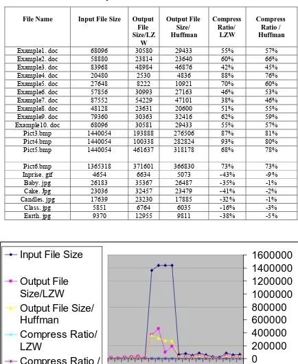
Firstly, with regards to compare between LZW and Huffman, Under the title (Group 1 Results), both LZW and Huffman will be used to compress and decompress different types of files, tries and results will be represented in a table, then figured in a chart to compare the efficiency of both programs in compressing and decompressing different types of files, conclusion and discussions are given at the end.

Figure 2.1 shows the results of using the

program in compressing different types of

files. In the chart, the dark blue curve

represents the input files sizes, the violet

curve represents the output files sizes when

compressed using LZW and the yellow

curve represents the output file size when

compressed using Huffman.

From table 2.1 and the figure 2.1, the

following conclusions and discussion can be

driven:

• LZW and Huffman give nearly results when used for compressing document or text files, as appears in the table and in the chart. The difference in the compression ratio is related to the different mechanisms of both in the compression process; which depends in LZW on replacing strings of characters with single codes, where in Huffman depends on representing individual characters with bit sequences.

• When LZW and Huffman are used to compress a binary file (all of its contents either 1 or 0), LZW gives a better compression ratio than Huffman. If you tried for example to compress one line of binary ( 00100101010111001101001010101110101...)

using LZW, you will arrive to a stage in which 5 or 6 consecutive binary digits are represented by a single new code ( 9 bits ), while in Huffman you will represents every individual binary digit with a bit sequence of 2 bits, so in Huffman the 5 or 6 binary digits which were represented in LZW by 9 bits are represented now with 10 or 12 bits; this decreases the compression ratio in the case of Huffman

appears in the chart for compressing bmp files, the results are somehow different. LZW seems to be better in compressing bmp files the Huffman; since it replaces sets of dots ( instead of strings of characters in text files ) with single codes; resulting in new codes that are useful when the dots that consists the image are repeated, while in Huffman, individual dots in the image are represented by bit sequences of a length depending on it’s probabilities. Because of the large different dots representing the image, the binary tree to be built is large, so the length of bit sequences which represents the individual dots increases, resulting in a less compression ratio compared to LZW compression.

- When LZW or Huffman is used to compress a file of type gif or type jpg, you will notice as in the table and in the chart that the compressed file size is larger than the original file size; this is due to being the images of these files are already compressed, so when compressed using LZW the number of the new output codes will increase, resulting in a file size larger than the original , while in Huffman the size of the binary tree built increases because of the less of probabilities, resulting in longer bit sequence that represent the individual dots of the image, so the compressed file size will be larger than the original . But because of being the new output code in LZW represented by 9 bits, while in Huffman the individual dot is represented with bits less than 9, this makes the resulting file size after compression in LZW larger than that in Huffman.

- Decompression operation is the opposite operation for compression; so the results will be the same as in compression.

Secondly, with regard to compare between LZW and HLZ,Under the title (Group 2 Results) both Huffman and LZW will be used to compress the same file, LZW compression then Huffman compression are applied consecutively to the same file or Huffman compression then LZW compression are applied to the same file, then a comparison between the two states will be done, conclusion and discussions are also given. The following table shows tries and results for group 2, will the chart in Fig. 2.2 represents these results.

From table 2.2 and figure 2.2, the following conclusions can be driven:

• Using LZH compression to compress a file of type: txt or bmp gives an improved compression ratio ( more than Huffman compression ratio, and LZW compression ratio ), this conclusion can be explained as follows: In the LZH compression, the file is firstly compressed using LZW, then compressed using Huffman, as it appeared from group 1 results that LZW gives good compression ratios for these types of files ( since it replaces strings of characters with single codes represented by 9 bits or more depending on the LZW output table), now the compressed file (.Lzw ) file which be compressed using Huffman, the (.Lzw ) file will be compressed perfectly by Huffman; since the phrases that are represented in LZW by 9 or more bits will now be represented by binary codes of 2, 3, 4 or more bits but still less than 8bits; this compresses the file more, and so improved compression ratios can be achieved using LZH compression.

• When LZH compression is used to compress file of types: TIFF, GIF or JPEG, it increases the output file size as it appears in the table and from the chart, this conclusion can be discussed as follows:

TIFF, GIF or JPEG files use LZW compression in their formats, and so when compressed using LZW, the output files sizes will be bigger the original, while when they are compressed using Huffman nearly good results can be achieved, so when a TIFF, GIF or JPEG file is firstly compressed with LZW resulting in a bigger file size using Huffman; so LZH compression is not efficient in the compression operation of these types of files.

When HLZ compression is used to compress files of types: Doc, Txt or Bmp, it gives a compression ratio that is less than the compression ratio obtained from as follows: Huffman compression replaces each byte in the input file with a binary code that is responded by 2, 3, 4 bits or more but still less than 8 bits, now when the compressed file using Huffman (.Huf) file is compressed using LZW phrases of binary will be composed and represented with codes of 9 or more bits which were in Huffman compressing these types of files.

output file than the original (since LZW is now used to compress an image that is really compressed using LZW); and so HLZ is not an efficient method in the compression operation of these types of files.

LZH is used to obtain highly compression ratios for the compression operation of files of types: Doc, Txt, Bmp, rather than HLZ.

Under this title some suggestions are given for increasing the performance of the compression these are below:

In order to increase the performance of compression, a comparison between LZW and Huffman to determine which is best in compressing a file is performed, and the output compressed file will be that of the less compression ratio, this can be used when the files is to be attached to an e-mail. Using LZW and Huffman for compression files of type: GIF or of type JPG can be studied and a program for good results can be built.

Finding a specific method for building the binary tree of Huffman, so as to decrease the length or determine the length of the bit sequences that represent the individual symbols can be studied and a program can be built for this purpose.

Other text compression and decompression algorithms can be studied and compared with the results of LZW and Huffman.

References

1. Compressed Image File Formats: JPEG, PNG, GIF, XBM, BMP, John Miano, August 1999 2. Introduction to Data Compression, Khalid

Sayood, Ed Fox (Editor), March 2000

3. Managing Gigabytes: Compressing and Indexing Documents and Images, Ian H H. Witten, Alistair Moffat, Timothy C. Bell , May 1999

4. Digital Image Processing, Rafael C. Gonzalez, Richard E. Woods, November 2001

5. The MPEG-4 Book

6. Fernando C. Pereira (Editor), Touradj Ebrahimi , July 2002

7. Apostolico, A. and Fraenkel, A. S. 1985. Robust Transmission of Unbounded Strings Using Fibonacci Representations. Tech. Rep. CS85-14, Dept. of Appl. Math., The

Weizmann Institute of Science, Rehovot, Sept.

8. Bentley, J. L., Sleator, D. D., Tarjan, R. E., and Wei, V. K. 1986. A Locally Adaptive Data Compression Scheme. Commun. ACM 29, 4 (Apr.), 320-330.

9. Connell, J. B. 1973. A Huffman-Shannon-Fano Code. Proc. IEEE 61,7 (July), 1046-1047.

10. Data Compression Conference (DCC '00), March 28-30, 2000, Snowbird, Utah

Table 2.1 Comparison between LZW and Huffman

File Name Input File Size Output

File Size/LZ

W

Output File Size/ Huffman

Compress Ratio/

LZW

Compress Ratio / Huffman

Example1. doc

68096 30580 29433 55% 57%

Example2. doc

58880 23814 23640 60% 66%

Example3. doc

83968 48984 46876 42% 45%

Example4. doc

20480 2530 4836 88% 76%

Example5. doc

27648 8222 10921 70% 60%

Example6. doc

57856 30993 27163 46% 53%

Example7. doc

87552 54229 47101 38% 46%

Example8. doc

48128 23631 20600 51% 55%

Example9. doc

79360 30363 62%32416 59%

Example10. doc

68096 30581 29433 55% 57%

Pict3.bmp

1440054 276506193888 87% 81%

Pict4.bmp

1440054 100338 282824 93% 80%

Pict5.bmp

4616371440054 318178 68% 78%

Pict6.bmp

1365318 371601 366830 73% 73%

Inprise. gif

4654 6634 5073 -43% -9%

Baby. jpg

26183 35367 26487 -35% -1%

Cake. Jpg

23036 32457 23479 -41% -2%

Candles. jpg

17639 23230 17885 -32% -1%

Class. jpg

5851 6764 6035 -16% -3%

Earth. jpg

9370 12955 9811 -38% -5%

-200000

0

200000

400000

600000

800000

1000000

1200000

1400000

1600000

1

4

7

10

13

16

19

Input File Size

Output File

Size/LZW

Output File Size/

Huffman

Compress Ratio/

LZW

Compress Ratio /

Huffman

Table 2.2 Comparison between LZW, Huffman, LZH and HLZ

compression ratios

-500000

0

500000

1000000

1500000

2000000

2500000

1

4

7

10

13

16

19

22

25

28

Input File Size

LZW

LZW%

HUF

HUF%

LZH

LZH%

HLZ

HLF%

Fig. 2.2 Comparison between LZH and HLZ compression ratios.

Input File Size LZW LZW %

HUF HU

F%

LZH LZH

%

HLZ

HLF %

1.doc

5705131216502 537542 359113 70 337749 72 487200 60 2.doc

659456 165288 75 157580 76 120529 82 137640 79 3.doc

491520 286957 42 306746 38 269146 45 361609 26 4.doc

436575 275193 37 162929 63 192012 56 168469 61 5.doc

71088 36721 48 44779 37 35468 50 53122 25 6.doc

45568 22092 52 22701 50 20452 55 25798 43 1.txt

3977 2571 35 2567 35 2865 28 3238 26 2.txt

12305 6715 45 7736 37 7028 43 9357 42 3.txt

20807 5757 72 13932 33 6177 70 10074 52 4.txt

20821 10725 48 13149 37 10990 47 14904 28 5.txt

39715 18936 52 24769 38 19183 52 27417 31 6.txt

25422 11335 55 16185 36 11703 54 17769 30 1.bmp

746082 286879 62 696526 37 273900 63 433512 42 2.bmp

83418 13402 84 27202 67 13735 84 18766 78 3.bmp

481080 606420 26 248644 48 361079 25 363798 24 4.bmp

222822 279781 26 215928 2499473 -12 363798 63 5.bmp

2137730 416950 80 610085 71 407932 81 564156 74 6.bmp

1440054 192930 87 1378239 16396864 -14 1970140 37 1.tif

84530 1110672 32 785693 11106727 -32 1085466 29 2.tif

1162804 1567927 35 1091514 13089636 -13 1536259 32 3.tif

775036 366622 53 468322 40 318365 59 450462 42 4.tif

1440180 2010465 40 1378329 16392024 -14 1960444 36 5.tif

82308 12862 84 26113 68 13007 84 18000 78 6.tif

481722 307993 36 429330 48 228563 53 248853 48 1.gif

85084 119442 40 85457 1023960 -20 121359 43 2.gif

18519 25425 37 18780 -1 22107 -19 26754 44 3.gif

63687 89482 41 64015 -1 76310 -20 90534 42 4.gif

62722 88180 41 63150 -1 76072 -21 89577 43 5.gif

83645 118375 42 84125 -1 101836 -22 119497 43 6.gif