Towards Compact and Fast Neural Machine Translation Using a Combined Method

Towards Compact and Fast Neural Machine Translation Using a

Combined Method

Xiaowei Zhang1,2_{, Wei Chen}1∗_{, Feng Wang}1,2_{, Shuang Xu}1 _{and Bo Xu}1 1_{Institute of Automation, Chinese Academy of Sciences, Beijing, China}

2_{University of Chinese Academy of Sciences, China}

{zhangxiaowei2015,w.chen,feng.wang,shuang.xu,boxu}@ia.ac.cn

Abstract

Neural Machine Translation (NMT) lays intensive burden on computation and memory cost. It is a challenge to de-ploy NMT models on the devices with limited computation and memory budgets. This paper presents a four stage pipeline to compress model and speed up the decod-ing for NMT. Our method first introduces a compact architecture based on convo-lutional encoder and weight shared em-beddings. Then weight pruning is ap-plied to obtain a sparse model. Next, we propose a fast sequence interpolation ap-proach which enables the greedy decod-ing to achieve performance on par with the beam search. Hence, the time-consuming beam search can be replaced by simple greedy decoding. Finally, vocabulary se-lection is used to reduce the computation of softmax layer. Our final model achieves 10×speedup, 17× parameters reduction,

<35MB storage size and comparable per-formance compared to the baseline model.

1 Introduction

Neural Machine Translation (NMT) ( Kalchbren-ner and Blunsom, 2013; Sutskever et al., 2014;

Bahdanau et al., 2015) has recently gained popu-larity in solving the machine translation problem. Although NMT has achieved state-of-the-art per-formance for several language pairs (Jean et al.,

2015;Wu et al.,2016), like many other deep learn-ing domains, it is both computationally intensive and memory intensive. This leads to a challenge of deploying NMT models on the devices with lim-ited computation and memory budgets.

∗

*Corresponding author

Numerous approaches have been proposed for compression and inference speedup of neural net-works, including but not limited to low-rank ap-proximation (Denton et al., 2014), hash function (Chen et al., 2015), knowledge distillation ( Hin-ton et al.,2015), quantization (Courbariaux et al.,

2015;Han et al.,2016;Zhou et al.,2017) and spar-sification (Han et al.,2015;Wen et al.,2016).

Weight pruning and knowledge distillation have been proved to be able to compress NMT mod-els (See et al., 2016;Kim and Rush, 2016; Fre-itag et al.,2017). The above methods reduce the parameters from a global perspective. However, embeddings dominate the parameters in a rela-tively compact NMT model even if subword ( Sen-nrich et al., 2016) (typical about 30K) is used. Character-aware methods (Ling et al., 2015; Lee et al.,2016) have fewer embeddings while suffer from slower decoding speed (Wu et al.,2016). Re-cent work byLi et al.(2016) has shown that weight sharing can be adopted to compress embeddings in language model. We are interested in applying embeddings weight sharing to NMT.

As for decoding speedup,Gehring et al.(2016);

Kalchbrenner et al. (2016) tried to improve the parallelism in NMT by substituting CNNs for RNNs .Kim and Rush(2016) proposed sequence-level knowledge distillation which allows us to replace beam search with greedy decoding. Gu et al. (2017) exploited trainable greedy decoding by the actor-critic algorithm (Konda and Tsitsiklis,

2002).Wu et al.(2016) evaluated the quantized in-ference of NMT. Vocabulary selection (Jean et al.,

2015;Mi et al., 2016; L’Hostis et al., 2016) was commonly used to speed up the softmax layer. Search pruning was also applied to speed up beam search (Hu et al., 2015; Wu et al., 2016;Freitag and Al-Onaizan,2017). Compared to search prun-ing, the speedup of greedy decoding is more at-tractive. Knowledge distillation improves the

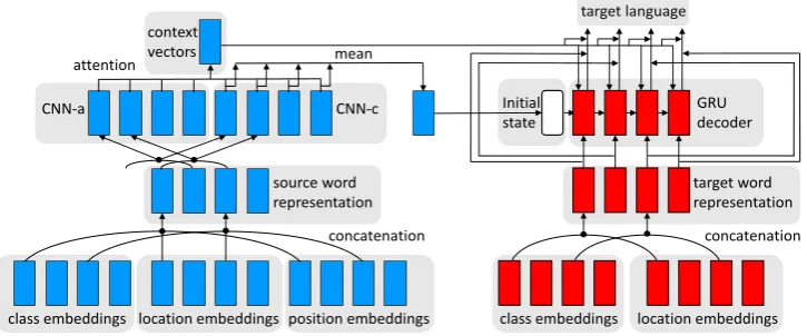
target language

concatenation

class embeddings location embeddings position embeddings class embeddings location embeddings Initial

state

GRU decoder

source word representation

target word representation

CNN-a CNN-c

mean attention

context vectors

concatenation

Figure 1: Our network architecture. The 2-component word representation contains class embeddings and location embed-dings. Position embeddings are concatenated to convey the absolute positional information of each source word.

formance of greedy decoding while the method needs to run beam search over the training set, and therefore results in inefficiency for tens of millions of corpus. The trainable greedy decoding using a relatively sophisticated training procedure. We prefer a simple and fast approach that allows us to replace beam search with the greedy search.

In this work, a novel approach is proposed to improve the performance of greedy decoding di-rectly and the embeddings weight sharing is intro-duced into NMT. We investigate the model com-pression and decoding speedup for NMT from the views of network architecture, sparsification, computation and search strategy, and test the per-formance of their combination. Specifically, we present a four stage pipeline for model compres-sion and decoding speedup. Firstly, we train a compact NMT model based on convolutional coder and weight sharing. The convolutional en-coder works well with smaller model size and is robust for pruning. Weight sharing further reduces the number of embeddings by several folds. Then weight pruning is applied to get a sparse model. Next, we propose fast sequence interpolation to improve the performance of greedy decoding di-rectly. This approach uses batched greedy decod-ing to obtain samples and therefore is more effi-cient thanKim and Rush(2016). Finally, we use vocabulary selection to reduce the computation of the softmax layer. Our final model achieves 10× speedup, 17×parameters reduction,<35MB stor-age size and comparable performance compared to the baseline model.

2 Method

2.1 Compact Network Architecture

Our network architecture is illustrated in Figure1. This architecture works well with fewer parame-ters, which allows us to match the performance of the baseline model at lower capacity. The convo-lutional encoder is similar toGehring et al.(2016), which consists of two convolutional neural net-works:CNN-afor attention score computation and

CNN-cfor the conditional input to be fed to the de-coder. The CNNs are constructed by blocks with residual connections (He et al., 2015). We use therelu61_{non-linear activation function instead of}

tanh in Gehring et al. (2016) and achieve better training stability.

To compress the embeddings, the cluster based 2-component word representation is intro-duced: we cluster the words into C classes by

word2vector2 _{(Mikolov et al., 2013), and each} class contains up to L words. Then the con-ventional embedding lookup table is replaced by

C +L unique vectors. For each word, we first do a lookup from C class embeddings according to which cluster the word belongs, next we do another lookup from L location embeddings ac-cording to the location of the word. We concate-nate the results of the two embedding lookup as the 2-component word representation. As a result, the number of embeddings is reduced from about

C×LtoC+L. Referring toGehring et al.(2016), position embeddings are concatenated to convey the absolute positional information of each source word within a sentence.

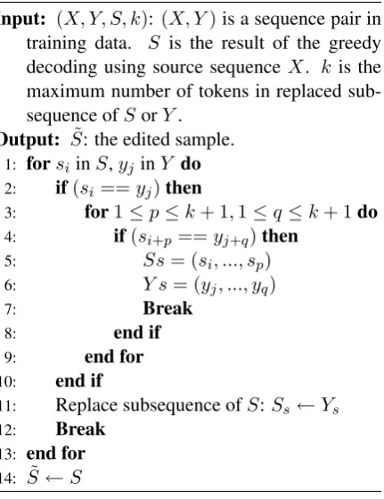
Reference (Y):

Sample (S):

Interpolated Sample:

replace

the official said the grenade explosion did not cause any casualties or damage .

the official said the grenade blast did not cause any casualties or damage .

the official said the grenade blast did not cause any death or injury nor any damage .

Boundary words

Figure 2:Editing operation. We search for subsequences with the same boundary words betweenSandY. The words within the boundary words can be different. Then we replace the subsequence inSby the subsequence inY.

2.2 Weight Pruning

Then the iterative pruning (Han et al.,2015) is ap-plied to obtain a sparse network, which allows us to use sparse matrix storage. In order to further re-duce the storage size, most sparse matrix index of our pruned model is stored usinguint8anduint16

depend on the matrix dimension.

2.3 Fast Sequence Interpolation

Let (X, Y) be a source-target sequence pair. Given X as input,S is the corresponding greedy decoding result using a well trained model. Then we make two assumptions:

(1) Let S˜ be a sequence close to S. If training with(X,S˜),S˜will replaceSto become the result of greedy decoding with a probabilityP( ˜S, S). (2) The following relationship holds:

P( ˜S, S)∝sim( ˜S, S) sim( ˜S, S)> sim(Y, S)

wheresimis a function measuring closeness such as edit-distance. IfS˜has higher evaluation metric3 (we write asE) thanS, according to (2) we have:

P( ˜S, S)> P(Y, S) E( ˜S, Y)> E(S, Y)

We note that usingS˜as a label is more attractive than Y for improving the performance of greedy decoding. The reason is that S and Y are often quite different (Kim and Rush,2016), resulting in a relatively lowP(Y, S). We bridge the gap be-tween S and Y by interpolating inner sequence between them. Specifically, weeditS towardY, which can be seen as interpolation. Editing is a heuristic operation as illustrated in Figure2. Con-cretely, letSsbe a subsequence ofS and letYsbe

3_{We use smoothed sentence-level BLEU (Chen and}

Cherry,2014).

Algorithm 1 Editing algorithm of fast sequence interpolation.

Input: (X, Y, S, k):(X, Y)is a sequence pair in training data. S is the result of the greedy decoding using source sequenceX. k is the maximum number of tokens in replaced sub-sequence ofSorY.

Output: S˜: the edited sample. 1: forsiinS,yj inY do 2: if(s_i ==y_j)then

3: for1≤p≤k+ 1,1≤q≤k+ 1do 4: if(si+p==yj+q)then

5: Ss= (s_i, ..., s_p) 6: Y s= (y_j, ..., y_q)

7: Break

8: end if 9: end for 10: end if

11: Replace subsequence ofS:Ss←Ys 12: Break

13: end for 14: S˜←S

a subsequence ofY. Given that:

      

S = (s0, ..., sp, Ss, sq, ..., sn) Y = (y0, ..., sp, Ys, sq, ..., ym)

length(Ss)6k

length(Ys)6k

wherekis the length limit ofSs andYs. The

in-terpolated sampleS˜has the following form:

˜

S = (s0, ..., sp, Ys, sq, ..., sn)

To obtain the target sequenceY˜ for training, we substituteS˜forY according to the following rule:

˜ Y =

_˜

S E( ˜S, Y)−E(S, Y)> ε Y otherwise

whereεaims to ensure the quality ofS˜. We define

over the training set. In summary, the following procedure is done iteratively: (1) get a new batch of(X, Y), (2) run batched greedy decoding onX, (3) editSto obtainS˜, (4) getY˜ according to the substitution rule, (5) train on the batched(X,Y˜).

2.4 Vocabulary Selection

We use word alignment4 _{(Dyer et al., 2013) to} build a candidate dictionary. For each source word, we build a list of candidate target words. When decoding, topncandidates of each word are merged to form a short-list for softmax layer. We do not apply vocabulary selection in training.

3 Experiments

3.1 Setup

Datasets and Evaluation Metrics: We eval-uate these approaches on two pairs of lan-guages: English-German and Chinese-English. Our English-German data comes from WMT’145_. The training set consists of 4.5M sentence pairs with 116M English words and 110M German words. We choose newstest2013 as the develop-ment set and newstest2014 as the test set. The Chinese-English training data consists of 1.6M pairs with 34M Chinese words and 38M English words. We chooseNIST 2002as the development set andNIST 2005as the test set.

For the two translation task, top 50K and 30k most frequent words are kept respectively. The rest words are replaced with UNK. We only use sentences of length up to 50 symbols. We do not use any UNK handling methods for fair compar-ison. The evaluation metric is case-insensitive BLEU (Papineni et al.,2002) as calculated by the

multi-bleu.perlscript.

Hyper-parameters: For the baseline model, we use a 2-layer bidirectional GRU encoder (1 layer in each direction) and a 1-layer GRU decoder. In

BaselineL, the embedding size is 512 and the hid-den size is 1024. InBaselineS, the embedding size is 256 and the hidden size is 512. Our baseline models are similar to the architecture in DL4MT6_. For the convolutional encoder model, 512 hidden units are used for the 6-layer CNN-a, and 256 hid-den units are used for the 8-layer CNN-c. The em-bedding size is 256. The hidden size of the

de-4_{https://github.com/clab/fast align} 5_{http://statmt.org/wmt14}

6_{https://github.com/nyu-dl/dl4mt-tutorial}

0.05 0.10 0.15 0.20 0.25 0.30

threshold

15.0 15.5 16.0 16.5 17.0 17.5 18.0 18.5 19.0

BLEU

BLEU(k=2)

BLEU(k=3)

0.0 0.1 0.2 0.3 0.4 0.5 0.6

Substitution rate

substitution rate(k=2)

substitution rate(k=3)

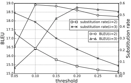
Figure 3: The performance and thesubstitution rateofFSI on English-German (newstest2013) development set with varying thresholdεand subsequence length limitk.

coder is 512. The kernel width in CNNs is 3. The number of clusters for both source and target vo-cabulary is 6. The editing rule for fast sequence interpolation is detailed in Algorithm 1. We use the top 50 candidates for each source word in vo-cabulary selection. The initial dropout rate is 0.3, and gradually decreases to 0 as the pruning rate increases. We use AdaDelta optimizer and clip the norm of the gradient to be no more than 1. Our methods are implemented with TensorFlow7 (Abadi et al.,2015). We run one sentence decod-ing for all models under the same computdecod-ing envi-ronment8_.

3.2 Results and Discussions

Our experimental results are summarized in Ta-ble1. The convolutional encoder model matches the performance of the GRU encoder model with about 2× fewer parameters. Combining with embeddings weight sharing results in a compact model that has about 3.5×fewer parameters than the baseline model. After pruning 80% of the weights, we reduce the parameters by about 17× with only a decrease of 0.2 BLEU. The storage size of the final models is about 30MB, which is easily fit into the memory of a mobile device. We find that the pruning rate of embeddings is highest even if weight sharing is used. Furthermore, the pruning rate of CNN layers is higher than GRU layers. This reveals that the CNNs are more robust for pruning than RNNs. The pruning rate of each

7_{https://github.com/zxw866/CFNMT}

8_{We also test batched greedy decoding with a batch size}

English→German Chinese→English

Approach Params Storage BLEU_k:10/1 Tdec Params Storage BLEUk:10/1 Tdec

BaselineL 110m 423MB 17.84/16.23 5145 80m 305MB 32.47/28.89 1914

BaselineS 47m 179MB 15.81/14.02 4056 31m 121MB 30.95/26.68 1412

Conv-Enc 50m 193MB 18.17/16.35 4159 35m 135MB 32.72/29.13 1437

+EWS 31m 119MB 17.85/15.89 4096 23m 90MB 32.44/28.62 1413

+Prune 80% 6m 33MB 17.63/16.02 4112 5m 25MB 32.78/28.95 1484

+FSI 6m 33MB 17.63/17.21 776 5m 25MB 32.69/31.74 297

+VS 6m 33MB 17.61/17.18 512 5m 25MB 32.63/31.67 198

Table 1:Results on English-German (newstest2014) and Chinese-English (nist05) test sets.EWS: embeddings weights shar-ing.VS: vocabulary selection.FSI: fast sequence interpolation.k: beam size.T_dec: decoding time on the test set in seconds.

Pruned models are saved as compressed sparse row (CSR) format with low bit index. Decoding runs on CPU in a preliminary implementation with TensorFlow, sparse matrix multiplication is unused for pruned models. After applyingFSI, beam search with a beam size 10 is replaced bygreedy decodingwhen recording Tdec.

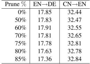
Prune% EN→DE CN→EN

0% 17.85 32.44

50% 17.83 32.47

60% 17.91 32.55

70% 17.81 32.65

75% 17.78 32.81

80% 17.63 32.78

85% 17.36 32.84

Table 2: BLEU on test sets with varying pruning rate. Model config:Conv Encoder+EWS.

class number EN→DE CN→EN

225 15.85 30.44

10 17.83 32.78

6 18.85 34.44

4 18.96 34.60

2 19.11 34.71

Table 3: BLEU on development sets with varying class number. Model config:Conv Encoder.

layer and the performance with increasing pruning rate are detailed in Figure 4. The compact archi-tecture reduces the decoding time by only 20%. The reason is that the decoding time is dominated by the softmax layer. After applying fast sequence interpolation, we replace beam search with greedy decoding, which results in a speedup of over5× with little loss in performance. We find that the details of the editing rules have little effect onFSI. Because we only accept S˜ that BLEU improved by more than the thresholdε, otherwise we choose the gold target sequence. Figure3shows that ap-propriatesubstitution rateis important for fast se-quence interpolation. We conjecture that edited samples are still worse than gold target sequences, and therefore relatively high substitution rate may

0% 10% 20% 30% 40% 50% 60% 70% 80% 90% 100%

Convolution Layer

GRU Layer FC Layer Embeddings Softmax Weights

Remaining Parameters Pruned Parameters

Figure 4:Pruning rate of different layers.

lead to instability in training. The speedup of vo-cabulary selection is only about 30%. It shows that the softmax layer no longer dominates the decod-ing time when usdecod-ing greedy search.

4 Conclusion and Future Work

We investigate the model compression and de-coding speedup for NMT from the views of net-work architecture, sparsification, computation and search strategy, and verify the performance on their combination. A novel approach is proposed to improve the performance of greedy decoding and the embeddings weight sharing is introduced into NMT. In the future, we plan to integrate weight quantization into our method.

Acknowledgments

References

Martłn Abadi, Paul Barham, Jianmin Chen, Zhifeng Chen, Andy Davis, Jeffrey Dean, Matthieu Devin, and et al Sanjay Ghemawat. 2015. Tensorflow: A system for large-scale machine learning. arXiv preprint arXiv:1605.08695.

D. Bahdanau, K. Cho, and Y. Bengio. 2015. Neural machine translation by jointly learning to align and translate. In ICLR.

Boxing Chen and Colin Cherry. 2014. A systematic comparison of smoothing techniques for sentence-level BLEU. In Proceedings of the Ninth Workshop on Statistical Machine Translation.

Wenlin Chen, James T Wilson, Stephen Tyree, Kilian Q Weinberger, and Yixin Chen. 2015. Compressing neural networks with the hashing trick. In ICML. Matthieu Courbariaux, Yoshua Bengio, and Jean-Pierre

David. 2015. Low precision arithmetic for deep learning.In ICLR.

Emily L Denton, Wojciech Zaremba, and Yann LeCun Joan Bruna, and Rob Fergus. 2014. Exploiting lin-ear structure within convolutional networks for effi-cient evaluation. In NIPS.

Chris Dyer, Victor Chahuneau, and Noah A. Smith. 2013. A simple, fast, and effective reparameteriza-tion of IBM model 2. In NAACL.

Markus Freitag and Yaser Al-Onaizan. 2017. Beam search strategies for neural machine translation.

arXiv preprint arXiv:1702.01806.

Markus Freitag, Yaser Al-Onaizan, and Baskaran Sankaran. 2017. Ensemble distillation for neural machine translation. arXiv preprint arXiv:1702.01802.

Jonas Gehring, Michael Auli, David Grangierm, and Yann N. Dauphin. 2016. A convolutional encoder model for neural machine translation. arXiv preprint arXiv:1611 02344.

Jiatao Gu, Kyunghyun Cho, and Victor O.K.Li. 2017. Trainable greedy decoding for neural machine trans-lation. arXiv preprint arXiv:1702.02429.

Song Han, Huizi Mao, and William J Dally. 2016. Deep compression: Compressing deep neural net-works with pruning, trained quantization and huff-man coding. In ICLR.

Song Han, Jeff Pool, John Tran, and William J. Dally. 2015. Learning both weights and connections for efficient neural networks. In NIPS.

Kaiming He, Xiangyu Zhang, Shaoqing Ren, and Jian Sun. 2015. Deep residual learning for image recog-nition.In CVPR.

Geoffrey Hinton, Oriol Vinyals, and Jeff Dean. 2015. Distilling the knowledge in a neural network. In NIPS Workshop.

Xiaoguang Hu, Wei Li, Xiang Lan, Hua Wu, and Haifeng Wang. 2015. Improved beam search with constrained softmax for NMT.In MT Summit.

S. Jean, K. Cho, R. Memisevic, and Y. Bengio. 2015. On using very large target vocabulary for neural ma-chine translation. In ACL.

Kalchbrenner and Blunsom. 2013. Recurrent continu-ous translation models. In EMNLP.

Nal Kalchbrenner, Lasse Espeholt, Karen Simonyan, Aaron van den Oord, Alex Graves, and Koray Kavukcuoglu. 2016. Neural machine translation in linear time. arXiv preprint arXiv:1610.10099.

Yoon Kim and Alexander M. Rush. 2016. Sequence-level knowledge distillation.In EMNLP.

VR Konda and JN Tsitsiklis. 2002. On actor-critic al-gorithms. Siam Journal on Control & Optimization. Jason Lee, Kyunghyun Cho, and Thomas Hofmann. 2016. Fully character-level neural machine trans-lation without explicit segmentation. arXiv preprint arXiv:1610.03017.

Gurvan L’Hostis, David Grangier, and Michael Auli. 2016. Vocabulary selection strategies for neural ma-chine translation. arXiv preprint arXiv:1610.00072.

Xiang Li, Tao Qin, Jian Yang, and Tie-Yan Liu. 2016. LightRNN: Memory and computation-efficient re-current neural networks.In NIPS.

Wang Ling, Isabel Trancoso, Chris Dyer, and Alan W Black. 2015. Character-based neural machine trans-lation.arXiv preprint arXiv:1511.04586.

Haitao Mi, Zhiguo Wang, and Abe Ittycheriah. 2016. Vocabulary manipulation for neural machine trans-lation.In ACL.

Tomas Mikolov, Kai Chen, Greg Corrado, and Jeffrey Dean. 2013. Efficient estimation of word represen-tations in vector space.In ICLR Workshop.

Kishore Papineni, Salim Roukos, Todd Ward, and Wei-Jing Zhu. 2002. BLEU: a method for automatic evaluation of machine translation.In ACL.

Abigail See, Minh-Thang Luong, and Christopher D. Manning. 2016. Compression of neural machine translation models via pruning. In CoNLL.

Rico Sennrich, Barry Haddow, and Alexandra Birch. 2016. Neural machine translation of rare words with subword units. In ACL.

Yonghui Wu, Mike Schuster, Zhifeng Chen, Quoc V Le, and Wolfgang Macherey Mohammad Norouzi, Maxim Krikun, Yuan Cao, Qin Gao, and et al. Klaus Macherey. 2016. Googles neural machine translation system: bridging the gap between hu-man and machine translation. arXiv preprint arXiv:1609.08144.